Concept explainers
Videos
Perform the same computation as in Sec. 32.1, but use
To calculate: The concentration of the distributed-parameter system equations for
Answer to Problem 1P
Solution: The concentration of equations for
Explanation of Solution
Given Information:
The distributed-parameter system depicts chemical modelling being subjected to first order decay and the tank is mixed well vertically and laterally.
Apply finite length of segment,
Here,
is the volume,
is the flow rate,
is the concentration,
is the dispersion coefficient,
is the tank’s cross-sectional area, and
is the first order decay coefficient.
Calculation:
Substitute centred finite differences for the first and the second derivatives in equation (1) to develop steady-state solution,
Further simplify the equation,
And,
Also,
Solve the equation (2),
Substitute
Hence, the required first equation is
Solve the equation (3),
Substitute
Hence, the required middle equation is
Substitute
in middle equation,
Substitute
Substitute
Substitute
Substitute
in middle equation,
Substitute
in middle equation,
Substitute
in middle equation,
Substitute
in middle equation,
Solve equation (4) for last equation,
Substitute
Hence, the required last equation is
Write all the equations in matrix form,
Express the matrix in tri-diagonal form,
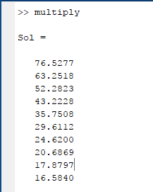
Use MATLAB to solve the above matrix.
The output of the program is given below.
Want to see more full solutions like this?
Chapter 32 Solutions
EBK NUMERICAL METHODS FOR ENGINEERS


- 3. Using the trial function uh(x) = a sin(x) and weighting function wh(x) = b sin(x) find an approximate solution to the following boundary value problems by determining the value of coefficient a. For each one, also find the exact solution using Matlab and plot the exact and approximate solutions. (One point each for: (i) finding a, (ii) finding the exact solution, and (iii) plotting the solution) a. (U₁xx - 2 = 0 u(0) = 0 u(1) = 0 b. Modify the trial function and find an approximation for the following boundary value problem. (Hint: you will need to add an extra term to the function to make it satisfy the boundary conditions.) (U₁xx - 2 = 0 u(0) = 1 u(1) = 0arrow_forwardFrom the following graph identify the steady-state maximum force. 1.2 1 0.8 0.6 0.4 0.2 0 Electical Power 1 Force vs. Time 2 Time (s) m 4 5arrow_forwardThe natural exponential function can be expressed by . Determine e2by calculating the sum of the series for:(a) n = 5, (b) n = 15, (c) n = 25For each part create a vector n in which the first element is 0, the incrementis 1, and the last term is 5, 15, or 25. Then use element-by-element calculations to create a vector in which the elements are . Finally, use the MATLAB built-in function sum to add the terms of the series. Compare thevalues obtained in parts (a), (b), and (c) with the value of e2calculated byMATLAB.arrow_forward
- Given: Time, t (s) 0 2 4 6 8 10 Position, x (m) 0 0 0.7 1.8 3.4 5.1 6.3 Using Centered-Finite Difference Method, find: find the velocities 12 14 16 7.3 8.0 8.4arrow_forwardFor the DE: dy/dx=2x-y y(0)=2 with h=0.2, solve for y using each method below in the range of 0 <= x <= 3: Q1) Using Matlab to employ the Euler Method (Sect 2.4) Q2) Using Matlab to employ the Improved Euler Method (Sect 2.5 close all clear all % Let's program exact soln for i=1:5 x_exact(i)=0.5*i-0.5; y_exact(i)=-x_exact(i)-1+exp(x_exact(i)); end plot(x_exact,y_exact,'b') % now for Euler's h=0.5 x_EM(1)=0; y_EM(1)=0; for i=2:5 x_EM(i)=x_EM(i-1)+h; y_EM(i)=y_EM(i-1)+(h*(x_EM(i-1)+y_EM(i-1))); end hold on plot (x_EM,y_EM,'r') % Improved Euler's Method h=0.5 x_IE(1)=0; y_IE(1)=0; for i=2:1:5 kA=x_IE(i-1)+y_IE(i-1); u=y_IE(i-1)+h*kA; x_IE(i)=x_IE(i-1)+h; kB=x_IE(i)+u; k=(kA+kB)/2; y_IE(i)=y_IE(i-1)+h*k; end hold on plot(x_IE,y_IE,'k')arrow_forwardIntegrate the function X^2+2*x on the interval 0 to 3 with a step size of .5 using the trapezoid rule.arrow_forward
- Use the graphical method to find the optimal solution for the following LP equations: Min Z=10 X1 + 25 X2 Subject to X1220, X2 ≤40 ,XI +X2 ≥ 50 X1, X2 ≥ 0.arrow_forward25.18 The following is an initial-value, second-order differential equation: d²x + (5x) dx + (x + 7) sin (wt) = 0 dt² dt where dx (0) (0) = 1.5 and x(0) = 6 dt Note that w= 1. Decompose the equation into two first-order differential equations. After the decomposition, solve the system from t = 0 to 15 and plot the results of x versus time and dx/dt versus time.arrow_forwardFind the three unknown on this problems using Elimination Method and Cramer's Rule. Attach your solutions and indicate your final answer. Problem 1. 7z 5y 3z 16 %3D 3z 5y + 2z -8 %3D 5z + 3y 7z = 0 Problem 2. 4x-2y+3z 1 *+3y-4z -7 3x+ y+2z 5arrow_forward
- Calculate the value of the first order derivative at the point x=0.2 with a single finite difference formula using all the following values. 0.1 0.2 0.3 0.4 f(x) 0.000 000 0.078 348 0.138 910 0.192 916 0.244981arrow_forwardSolve the following differential equation for axial deformation of a bar of length 12mm using Galerkin Weighted Residual method 2022/09/ d² dx² = -0.75(4- x)² One end of the bar is fixed whereas the displacement is 12 mm at the other end of the bar. You may use Matlab for computations. Use the trial function û(x) = Co + ₂x + ₂x²arrow_forward(3) For the given boundary value problem, the exact solution is given as = 3x - 7y. (a) Based on the exact solution, find the values on all sides, (b) discretize the domain into 16 elements and 15 evenly spaced nodes. Run poisson.m and check if the finite element approximation and exact solution matches, (c) plot the D values from step (b) using topo.m. y Side 3 Side 1 8.0 (4) The temperature distribution in a flat slab needs to be studied under the conditions shown i the table. The ? in table indicates insulated boundary and Q is the distributed heat source. I all cases assume the upper and lower boundaries are insulated. Assume that the units of length energy, and temperature for the values shown are consistent with a unit value for the coefficier of thermal conductivity. Boundary Temperatures 6 Case A C D. D. 00 LEGION Side 4 z episarrow_forward
 Principles of Heat Transfer (Activate Learning wi...Mechanical EngineeringISBN:9781305387102Author:Kreith, Frank; Manglik, Raj M.Publisher:Cengage Learning