Concept explainers
Videos
Repeat Example 30.1, but use the midpoint method to generate your solution.
To calculate: The solution of the one-dimensional heat conduction equation using midpoint method for a thing rod of length
Answer to Problem 1P
Solution: The desired result is as shown below.
Explanation of Solution
Given Information:
The expression of the temperature distribution of long, thin rod is,
Calculation:
Calculate
and
The expression of temperature,
Rewrite the above equation,
Rewrite the above equation,
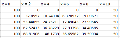
Substitute the value at t = 0.1 s for the node at x = 2 cm,
The results at the other interior points are,
Therefore,
Next,
And,
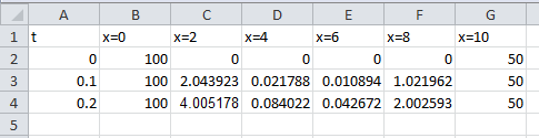
The value at t = 0.2 s; the interior points are four are,
Therefore,
Next,
And,
The Midpoint method in this subpart is,
And,
Use
predictor is calculating as follow:
Slop-midpoint,
Calculate corrector,
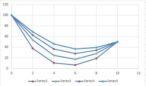
Use Excel to create the table as follow,
Use excel to solve this problem.
Step 1 Open the excel-spreadsheet and then press Alt+F11.
Step 2 Then there is a window opened in which write the coding to find optimal solution is as below,
Step 3 Now press F5, a new popup window will appear as shown below.
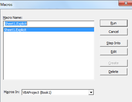
Step 4 Press run after selecting the program name, the desired result will be,
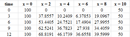
The flotation of the table is,
Want to see more full solutions like this?
Chapter 30 Solutions
EBK NUMERICAL METHODS FOR ENGINEERS


- Consider the function p(x) = x² - 4x³+3x²+x-1. Use Newton-Raphson's method with initial guess of 3. What's the updated value of the root at the end of the second iteration? Type your answer...arrow_forwardWrite a brief (a few sentences) discussion about the significance of each of the following in regards to an iterative CFD solution: (a) initial conditions, (b) residual, (c) iteration, and (d) postprocessing.arrow_forward(NUMBER 1.) solve for Lm, Pm, and Wm. I’ve attached a reference image with the solution method, I just need clarification.arrow_forward
- I need a clear step by step answer please with the simplest method Thank you :)arrow_forward25.18 The following is an initial-value, second-order differential equation: d²x + (5x) dx + (x + 7) sin (wt) = 0 dt² dt where dx (0) (0) = 1.5 and x(0) = 6 dt Note that w= 1. Decompose the equation into two first-order differential equations. After the decomposition, solve the system from t = 0 to 15 and plot the results of x versus time and dx/dt versus time.arrow_forwardFor the DE: dy/dx=2x-y y(0)=2 with h=0.2, solve for y using each method below in the range of 0 <= x <= 3: Q1) Using Matlab to employ the Euler Method (Sect 2.4) Q2) Using Matlab to employ the Improved Euler Method (Sect 2.5 close all clear all % Let's program exact soln for i=1:5 x_exact(i)=0.5*i-0.5; y_exact(i)=-x_exact(i)-1+exp(x_exact(i)); end plot(x_exact,y_exact,'b') % now for Euler's h=0.5 x_EM(1)=0; y_EM(1)=0; for i=2:5 x_EM(i)=x_EM(i-1)+h; y_EM(i)=y_EM(i-1)+(h*(x_EM(i-1)+y_EM(i-1))); end hold on plot (x_EM,y_EM,'r') % Improved Euler's Method h=0.5 x_IE(1)=0; y_IE(1)=0; for i=2:1:5 kA=x_IE(i-1)+y_IE(i-1); u=y_IE(i-1)+h*kA; x_IE(i)=x_IE(i-1)+h; kB=x_IE(i)+u; k=(kA+kB)/2; y_IE(i)=y_IE(i-1)+h*k; end hold on plot(x_IE,y_IE,'k')arrow_forward
- For the following system, perform only the first elimination using Gaussian Elimination with partial pivoting.arrow_forwardf(x)=-0.9x? +1.7x+2.5 Calculate the root of the function given below: a) by Newton-Raphson method b) by simple fixed-point iteration method. (f(x)=0) Use x, = 5 as the starting value for both methods. Use the approximate relative error criterion of 0.1% to stop iterations.arrow_forward2. Let p 19. Then 2 is a primitive root. Use the Pohlig-Hellman method to compute L2(14).arrow_forward
- Approximate solution of the initial value problem up to 3rd order using the Taylor series method. find it.arrow_forwardQ3) Find the optimal solution by using graphical method:. Max Z = x1 + 2x2 Subject to : 2x1 + x2 < 100 X1 +x2 < 80 X1 < 40 X1, X2 2 0arrow_forward3.1-6 DI 3.1-6. Use the graphical method to solve the problem: Maximize Z = 10x + 20x2, subject to -X + 2x, s 15 X1 + x2 < 12, 5x, + 3x s 45 and X 0, x2 2 0. 3.1-11 (a) and (b) only For (a), please specify: (1) Decision variables; (2) Objective function; (3) Constraints. MacBook Proarrow_forward
 Elements Of ElectromagneticsMechanical EngineeringISBN:9780190698614Author:Sadiku, Matthew N. O.Publisher:Oxford University Press
 Mechanics of Materials (10th Edition)Mechanical EngineeringISBN:9780134319650Author:Russell C. HibbelerPublisher:PEARSON
 Thermodynamics: An Engineering ApproachMechanical EngineeringISBN:9781259822674Author:Yunus A. Cengel Dr., Michael A. BolesPublisher:McGraw-Hill Education
 Control Systems EngineeringMechanical EngineeringISBN:9781118170519Author:Norman S. NisePublisher:WILEY
 Mechanics of Materials (MindTap Course List)Mechanical EngineeringISBN:9781337093347Author:Barry J. Goodno, James M. GerePublisher:Cengage Learning
 Engineering Mechanics: StaticsMechanical EngineeringISBN:9781118807330Author:James L. Meriam, L. G. Kraige, J. N. BoltonPublisher:WILEY