Concept explainers
Videos
(a)
Section 1:
The 20 simple random samples of size 5 and record the number of females in each sample.
(a)
Section 1:
Answer to Problem 13E
Solution: The partial output of the 20 simple random samples is shown below:
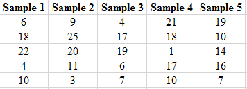
The number of females in each sample is shown below.
| Samples | Number of females | Samples | Number of females |
| Sample 1 | 2 | Sample 11 | 1 |
| Sample 2 | 1 | Sample 12 | 2 |
| Sample 3 | 2 | Sample 13 | 4 |
| Sample 4 | 3 | Sample 14 | 2 |
| Sample 5 | 1 | Sample 15 | 3 |
| Sample 6 | 2 | Sample 16 | 2 |
| Sample 7 | 3 | Sample 17 | 0 |
| Sample 8 | 1 | Sample 18 | 2 |
| Sample 9 | 1 | Sample 19 | 1 |
| Sample 10 | 2 | Sample 20 | 2 |
Explanation of Solution
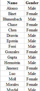
Step 1: Write the name and the gender of the club members in the Excel spreadsheet. The snapshot is shown below:
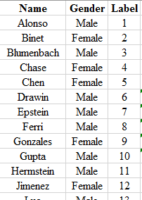
Step 2: Label each of the members using the numbers 1,2,⋯,25. The snapshot is shown below:
Step 3: Use the formula =RANDBETWEN(Bottom, Top) to generate a single set of

To find the number of female in each sample, the label of each female member is matched with the obtained random number of each set of sample and then the number of female is counted. The number of females obtained in each set of samples are shown in the below table.
| Samples | Number of females | Samples | Number of females |
| Sample 1 | 2 | Sample 11 | 1 |
| Sample 2 | 1 | Sample 12 | 2 |
| Sample 3 | 2 | Sample 13 | 4 |
| Sample 4 | 3 | Sample 14 | 2 |
| Sample 5 | 1 | Sample 15 | 3 |
| Sample 6 | 2 | Sample 16 | 2 |
| Sample 7 | 3 | Sample 17 | 0 |
| Sample 8 | 1 | Sample 18 | 2 |
| Sample 9 | 1 | Sample 19 | 1 |
| Sample 10 | 2 | Sample 20 | 2 |
To graph: The histogram for the number of females in each set of sample.
Explanation of Solution
Graph: To obtain the histogram for the obtained result in previous part, Excel is used. The below steps are followed to obtain the required histogram.
Step 1: The number of females varies from 0 to 4. The number of samples are calculated corresponding to each number of females. The number of samples with the same number of female members is clustered. The snapshot of the obtained table is shown below:
| Number of female members | Number of samples |
| 0 | 1 |
| 1 | 6 |
| 2 | 9 |
| 3 | 3 |
| 4 | 1 |
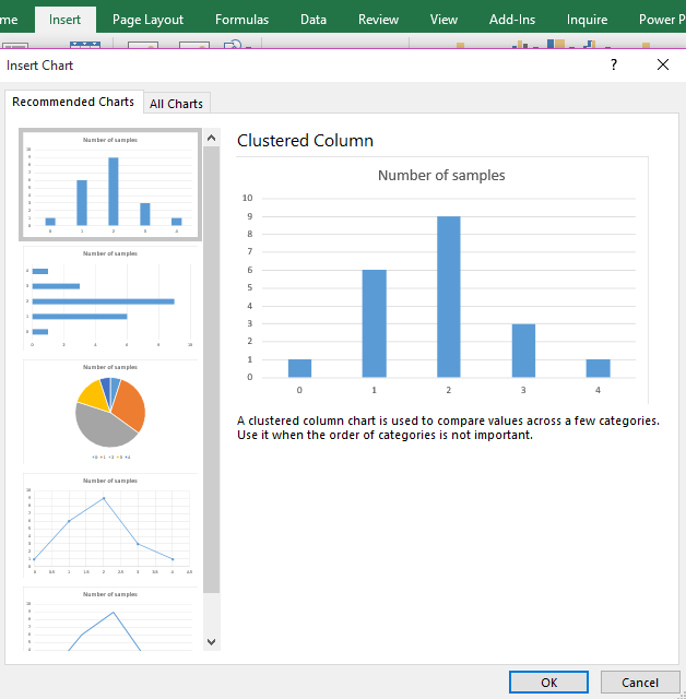
Step 2: Select the data set and go to insert and select the option of cluster column under the Recommended Charts. The screenshot is shown below:
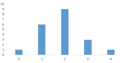
Step 3: Click on OK. The diagram is obtained as:
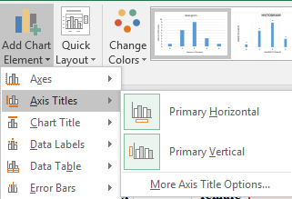
Step 4: Click on the chart area and select the option of “Primary Horizontal” and “Primary Vertical” axis under the “Add Chart Element” to add the axis title. The screenshot is shown below:
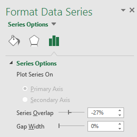
Step 5: Click on the bars of the diagrams and reduce the gap width to zero under the “Format Data Series” tab. The screenshot is shown below:
The obtained histogram is:
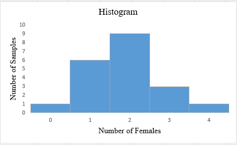
Interpretation: The obtained histogram for the number of females in each set of sample follows
To find: The average number of females in 20 samples.
Answer to Problem 13E
Solution: The average number of female is 1.85.
Explanation of Solution
Calculation:
The average number of females can be obtained by using the formula:
Average=Sum of(Number of female memebers×Number of samples)Total number of samples
Hence, the average number of females is calculated as:
Average=Sum of(Number of female memebers×Number of samples)Total number of samples=(0×1)+(1×6)+(2×9)+(3×3)+(4×1)20=1.85
Therefore, the average number of females in 20 samples is 1.85.
(b)
To explain: Whether the club members should be doubtful about the discrimination if any of the five tickets does not received by women.
(b)
Answer to Problem 13E
Solution: The club member should suspect the discrimination if any of the five tickets does not received by women.
Explanation of Solution
Want to see more full solutions like this?
Chapter 3 Solutions
Statistics: Concepts and Controversies


- To help consumers in purchasing a laptop computer, Consumer Reports calculates an overall test score for each computer tested based upon rating factors such as ergonomics, portability, performance, display, and battery life. Higher overall scores indicate better test results. The following data show the average retail price and the overall score for ten 13-inch models (Consumer Reports website, October 25, 2012). Brand & Model Price ($) Overall Score Samsung Ultrabook NP900X3C-A01US 1250 83 Apple MacBook Air MC965LL/A 1300 83 Apple MacBook Air MD231LL/A 1200 82 HP ENVY 13-2050nr Spectre XT 950 79 Sony VAIO SVS13112FXB 800 77 Acer Aspire S5-391-9880 Ultrabook 1200 74 Apple MacBook Pro MD101LL/A 1200 74 Apple MacBook Pro MD313LL/A 1000 73 Dell Inspiron I13Z-6591SLV 700 67 Samsung NP535U3C-A01US 600 63 a. Select a scatter diagram with price as the independent variable. b. What does the scatter diagram developed in part (a) indicate about the relationship…arrow_forwardTo the Internal Revenue Service, the reasonableness of total itemized deductions depends on the taxpayer’s adjusted gross income. Large deductions, which include charity and medical deductions, are more reasonable for taxpayers with large adjusted gross incomes. If a taxpayer claims larger than average itemized deductions for a given level of income, the chances of an IRS audit are increased. Data (in thousands of dollars) on adjusted gross income and the average or reasonable amount of itemized deductions follow. Adjusted Gross Income ($1000s) Reasonable Amount ofItemized Deductions ($1000s) 22 9.6 27 9.6 32 10.1 48 11.1 65 13.5 85 17.7 120 25.5 Compute b1 and b0 (to 4 decimals).b1 b0 Complete the estimated regression equation (to 2 decimals). = + x Predict a reasonable level of total itemized deductions for a taxpayer with an adjusted gross income of $52.5 thousand (to 2 decimals). thousand dollarsWhat is the value, in dollars, of…arrow_forwardK The mean height of women in a country (ages 20-29) is 63.7 inches. A random sample of 65 women in this age group is selected. What is the probability that the mean height for the sample is greater than 64 inches? Assume σ = 2.68. The probability that the mean height for the sample is greater than 64 inches is (Round to four decimal places as needed.)arrow_forward
- In a survey of a group of men, the heights in the 20-29 age group were normally distributed, with a mean of 69.6 inches and a standard deviation of 4.0 inches. A study participant is randomly selected. Complete parts (a) through (d) below. (a) Find the probability that a study participant has a height that is less than 68 inches. The probability that the study participant selected at random is less than 68 inches tall is 0.4. (Round to four decimal places as needed.) 20 2arrow_forwardPEER REPLY 1: Choose a classmate's Main Post and review their decision making process. 1. Choose a risk level for each of the states of nature (assign a probability value to each). 2. Explain why each risk level is chosen. 3. Which alternative do you believe would be the best based on the maximum EMV? 4. Do you feel determining the expected value with perfect information (EVWPI) is worthwhile in this situation? Why or why not?arrow_forwardQuestions An insurance company's cumulative incurred claims for the last 5 accident years are given in the following table: Development Year Accident Year 0 2018 1 2 3 4 245 267 274 289 292 2019 255 276 288 294 2020 265 283 292 2021 263 278 2022 271 It can be assumed that claims are fully run off after 4 years. The premiums received for each year are: Accident Year Premium 2018 306 2019 312 2020 318 2021 326 2022 330 You do not need to make any allowance for inflation. 1. (a) Calculate the reserve at the end of 2022 using the basic chain ladder method. (b) Calculate the reserve at the end of 2022 using the Bornhuetter-Ferguson method. 2. Comment on the differences in the reserves produced by the methods in Part 1.arrow_forward
- You are provided with data that includes all 50 states of the United States. Your task is to draw a sample of: o 20 States using Random Sampling (2 points: 1 for random number generation; 1 for random sample) o 10 States using Systematic Sampling (4 points: 1 for random numbers generation; 1 for random sample different from the previous answer; 1 for correct K value calculation table; 1 for correct sample drawn by using systematic sampling) (For systematic sampling, do not use the original data directly. Instead, first randomize the data, and then use the randomized dataset to draw your sample. Furthermore, do not use the random list previously generated, instead, generate a new random sample for this part. For more details, please see the snapshot provided at the end.) Upload a Microsoft Excel file with two separate sheets. One sheet provides random sampling while the other provides systematic sampling. Excel snapshots that can help you in organizing columns are provided on the next…arrow_forwardThe population mean and standard deviation are given below. Find the required probability and determine whether the given sample mean would be considered unusual. For a sample of n = 65, find the probability of a sample mean being greater than 225 if μ = 224 and σ = 3.5. For a sample of n = 65, the probability of a sample mean being greater than 225 if μ=224 and σ = 3.5 is 0.0102 (Round to four decimal places as needed.)arrow_forward***Please do not just simply copy and paste the other solution for this problem posted on bartleby as that solution does not have all of the parts completed for this problem. Please answer this I will leave a like on the problem. The data needed to answer this question is given in the following link (file is on view only so if you would like to make a copy to make it easier for yourself feel free to do so) https://docs.google.com/spreadsheets/d/1aV5rsxdNjHnkeTkm5VqHzBXZgW-Ptbs3vqwk0SYiQPo/edit?usp=sharingarrow_forward
- The data needed to answer this question is given in the following link (file is on view only so if you would like to make a copy to make it easier for yourself feel free to do so) https://docs.google.com/spreadsheets/d/1aV5rsxdNjHnkeTkm5VqHzBXZgW-Ptbs3vqwk0SYiQPo/edit?usp=sharingarrow_forwardThe following relates to Problems 4 and 5. Christchurch, New Zealand experienced a major earthquake on February 22, 2011. It destroyed 100,000 homes. Data were collected on a sample of 300 damaged homes. These data are saved in the file called CIEG315 Homework 4 data.xlsx, which is available on Canvas under Files. A subset of the data is shown in the accompanying table. Two of the variables are qualitative in nature: Wall construction and roof construction. Two of the variables are quantitative: (1) Peak ground acceleration (PGA), a measure of the intensity of ground shaking that the home experienced in the earthquake (in units of acceleration of gravity, g); (2) Damage, which indicates the amount of damage experienced in the earthquake in New Zealand dollars; and (3) Building value, the pre-earthquake value of the home in New Zealand dollars. PGA (g) Damage (NZ$) Building Value (NZ$) Wall Construction Roof Construction Property ID 1 0.645 2 0.101 141,416 2,826 253,000 B 305,000 B T 3…arrow_forwardRose Par posted Apr 5, 2025 9:01 PM Subscribe To: Store Owner From: Rose Par, Manager Subject: Decision About Selling Custom Flower Bouquets Date: April 5, 2025 Our shop, which prides itself on selling handmade gifts and cultural items, has recently received inquiries from customers about the availability of fresh flower bouquets for special occasions. This has prompted me to consider whether we should introduce custom flower bouquets in our shop. We need to decide whether to start offering this new product. There are three options: provide a complete selection of custom bouquets for events like birthdays and anniversaries, start small with just a few ready-made flower arrangements, or do not add flowers. There are also three possible outcomes. First, we might see high demand, and the bouquets could sell quickly. Second, we might have medium demand, with a few sold each week. Third, there might be low demand, and the flowers may not sell well, possibly going to waste. These outcomes…arrow_forward
 MATLAB: An Introduction with ApplicationsStatisticsISBN:9781119256830Author:Amos GilatPublisher:John Wiley & Sons Inc
 Probability and Statistics for Engineering and th...StatisticsISBN:9781305251809Author:Jay L. DevorePublisher:Cengage Learning
 Statistics for The Behavioral Sciences (MindTap C...StatisticsISBN:9781305504912Author:Frederick J Gravetter, Larry B. WallnauPublisher:Cengage Learning
 Elementary Statistics: Picturing the World (7th E...StatisticsISBN:9780134683416Author:Ron Larson, Betsy FarberPublisher:PEARSON
 The Basic Practice of StatisticsStatisticsISBN:9781319042578Author:David S. Moore, William I. Notz, Michael A. FlignerPublisher:W. H. Freeman
 Introduction to the Practice of StatisticsStatisticsISBN:9781319013387Author:David S. Moore, George P. McCabe, Bruce A. CraigPublisher:W. H. Freeman