
Concept explainers
Videos
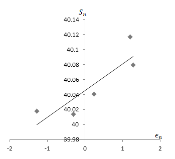
Simulate five sample trajectories of Eq.
Hint: For the
Equation
where
The five sample trajectories of the equation
Answer to Problem 1P
Solution:
The five sample trajectories for
The five sample trajectories for
For
Explanation of Solution
Given information:
The discrete model for change in the price of a stock over a time interval
The parameter values are
Highly volatile have a large value for
A sequence of numbers
Explanation:
The discrete model for change in the price of a stock over a time interval
Where
The parameter values are
Substitute the above values in the equation (1)
Here,
Thus, equation (1) becomes,
Now, to find the value of
By using the computer technology,
For
Substitute the values in equation (2)
For
Substitute the values in equation (2)
For
Substitute the values in equation (2)
For
Substitute the values in equation (2)
For
Substitute the values in equation (2)
Hence, the graph of trajectories for
Now, for the value
Here,
Thus, equation (1) becomes,
Now, to find the value of
By using computer technology,
For
Substitute the values in equation (3)
For
Substitute the values in equation (3)
For
Substitute the values in equation (3)
For
Substitute the values in equation (2)
For
Substitute the values in equation (3)
The graph of trajectories for
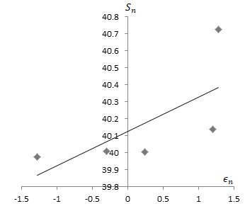
Since the approximation in the graph of trajectories for
Therefore, for
Want to see more full solutions like this?
Chapter 2 Solutions
DIFFERENTIAL EQUATIONS(LL) W/WILEYPLUS
Additional Math Textbook Solutions
Probability and Statistics for Engineers and Scientists
Thinking Mathematically (7th Edition)
Fundamentals of Differential Equations and Boundary Value Problems
A Survey of Mathematics with Applications (10th Edition) - Standalone book
Calculus for Business, Economics, Life Sciences, and Social Sciences (13th Edition)
Finite Mathematics for Business, Economics, Life Sciences and Social Sciences


- Find the equation of the regression line for the following data set. x 1 2 3 y 0 3 4arrow_forwardOlympic Pole Vault The graph in Figure 7 indicates that in recent years the winning Olympic men’s pole vault height has fallen below the value predicted by the regression line in Example 2. This might have occurred because when the pole vault was a new event there was much room for improvement in vaulters’ performances, whereas now even the best training can produce only incremental advances. Let’s see whether concentrating on more recent results gives a better predictor of future records. (a) Use the data in Table 2 (page 176) to complete the table of winning pole vault heights shown in the margin. (Note that we are using x=0 to correspond to the year 1972, where this restricted data set begins.) (b) Find the regression line for the data in part ‚(a). (c) Plot the data and the regression line on the same axes. Does the regression line seem to provide a good model for the data? (d) What does the regression line predict as the winning pole vault height for the 2012 Olympics? Compare this predicted value to the actual 2012 winning height of 5.97 m, as described on page 177. Has this new regression line provided a better prediction than the line in Example 2?arrow_forwardConsider a linear regression model for the decrease in blood pressure (mmHg) over a four-week period with muy=2.8+0.8x and standard deviation chi=3.2. The explanatory variable x is the number of servings fruits and vegetables in a calorie-controlled diet. What is the subpopulation mean when x = 7 servings per day?arrow_forward
- In an experiment, the independent variable is the percentage of hydrocarbons and the dependent variable is the purity of oxygen produced in a chemical distillation process that are present in the main condenser of the distillation unit. The simple linear regression and correlation analysis is performed in a sample of 9 observations. Results are as shown below: SSxx : 113.7356 SSyy = 0.5156 уу a = -4.2869 b = 0.0648 %3Darrow_forwardLasse has set up a model evaluating daily electricity prices using observations from the last year (price of electricity is the dependent variable). He has set up a test to verify whether data are stationary. The t-statistic for electricity price is equal to -5.2. What can he conclude?arrow_forwardA paper gives data on x = change in Body Mass Index (BMI, in kilograms/meter2) and y = change in a measure of depression for patients suffering from depression who participated in a pulmonary rehabilitation program. The table below contains a subset of the data given in the paper and are approximate values read from a scatterplot in the paper. BMI Change (kg/m²) Depression Score Change S = The accompanying computer output is from Minitab. Depression score change 15- 10- -0.5 S Fitted Line Plot Depression score change = 6.577 +5.440 BMI change 20- 5.30586 Coefficients T 0.0 0.5 -0.5 R-sq 25.96% - 1 Term Coef Constant 6.577 BMI change 5.440 % 0.5 BMI change 1.0 SE Coef 2.28 2.90 9 0 0.1 0.7 0.8 1 1.5 4 T-Value 2.88 1.87 Interpret this estimate. s is the typical amount by which the ---Select--- line. 4 5 Regression Equation Depression score change = 6.577 +5.440 BMI change P-Value 0.0164 0.0906 S 5.30586 25.96% R-Sq R-Sq (adj) 18.56% 8 (b) Give a point estimate of o. (Round your answer to…arrow_forward
 Calculus For The Life SciencesCalculusISBN:9780321964038Author:GREENWELL, Raymond N., RITCHEY, Nathan P., Lial, Margaret L.Publisher:Pearson Addison Wesley,
 Glencoe Algebra 1, Student Edition, 9780079039897...AlgebraISBN:9780079039897Author:CarterPublisher:McGraw Hill
 Algebra & Trigonometry with Analytic GeometryAlgebraISBN:9781133382119Author:SwokowskiPublisher:Cengage
 College AlgebraAlgebraISBN:9781305115545Author:James Stewart, Lothar Redlin, Saleem WatsonPublisher:Cengage Learning
 Functions and Change: A Modeling Approach to Coll...AlgebraISBN:9781337111348Author:Bruce Crauder, Benny Evans, Alan NoellPublisher:Cengage Learning