Videos
The dynamics of a forced spring-mass-damper system can be represented by the following second-order ODE:
where
(a)
To calculate: The displacement and velocity as a function of time for linear system where
Answer to Problem 49P
Solution:
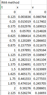
The first few solutions for displacement and velocity as a function of time for liner system is,
| t | x | v |
| 0 | 0 | 0 |
| 0.125 | 0.003836 | 0.060764 |
| 0.25 | 0.015019 | 0.117402 |
| 0.375 | 0.032976 | 0.169015 |
| 0.5 | 0.05703 | 0.214828 |
| 0.625 | 0.086414 | 0.254195 |
| 0.75 | 0.120289 | 0.286602 |
| 0.875 | 0.157759 | 0.311673 |
| 1 | 0.197891 | 0.329164 |
| 1.125 | 0.239729 | 0.338967 |
| 1.25 | 0.282313 | 0.341104 |
| 1.375 | 0.324691 | 0.335717 |
| 1.5 | 0.365939 | 0.323069 |
| 1.625 | 0.405171 | 0.303527 |
| 1.75 | 0.441553 | 0.277555 |
| 1.875 | 0.474314 | 0.245705 |
| 2 | 0.50276 | 0.208601 |
| 2.125 | 0.526274 | 0.16693 |
| 2.25 | 0.544332 | 0.121428 |
| 2.375 | 0.556503 | 0.072863 |
| 2.5 | 0.562454 | 0.02203 |
| 2.625 | 0.56195 | -0.03027 |
| 2.75 | 0.554859 | -0.08324 |
| 2.875 | 0.541146 | -0.13608 |
| 3 | 0.520874 | -0.18805 |
| 3.125 | 0.494199 | -0.23842 |
| 3.25 | 0.461364 | -0.28651 |
| 3.375 | 0.422694 | -0.33168 |
| 3.5 | 0.378588 | -0.37339 |
| 3.625 | 0.329513 | -0.41112 |
| 3.75 | 0.275993 | -0.44444 |
| 3.875 | 0.218601 | -0.47301 |
| 4 | 0.157952 | -0.49653 |
| 4.125 | 0.094688 | -0.5148 |
| 4.25 | 0.029475 | -0.52771 |
| 4.375 | -0.03701 | -0.53518 |
| 4.5 | -0.1041 | -0.53725 |
| 4.625 | -0.1711 | -0.53399 |
| 4.75 | -0.23738 | -0.52558 |
| 4.875 | -0.30229 | -0.51221 |
| 5 | -0.36524 | -0.49416 |
Explanation of Solution
Given Information:
The dynamic of a forced spring-mass-damper system is given as,
The values,
The initial condition,
Formula used:
The fourth-order RK method for
Where,
Calculation:
Consider the dynamic of a forced spring-mass-damper system,
As
Divide both the sides of above equation by m,
Now, substitute the values
For linear, substitute
Use VBA code for RK4 method as below to solve for x and v,
Code:
Output:
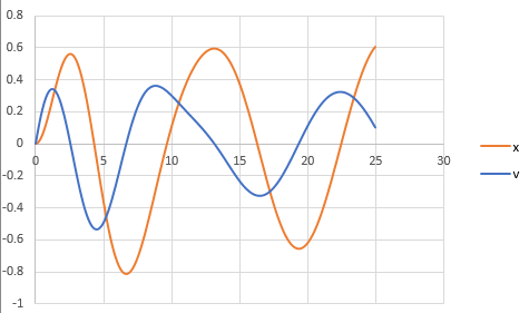
To draw the graph of the above results, follow the steps in excel sheet as given below,
Step 1: Select the cell from A4 to A205 and cell B4 to B205. Then, go to the Insert and select the scatter with smooth lines from the chart.
Step 2: Select the cell from A4 to A205 and cell C4 to C205. Then, go to the Insert and select the scatter with smooth lines from the chart.
Step 3: Select one of the graphs and paste it on another graph to merge the graphs.
The graph obtained is,
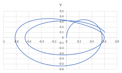
And, to draw the phase plane plot follow the steps as below,
Step 4: Select the column B and column C. Then, go to the Insert and select the scatter with smooth lines from the chart.
The graph obtained is,
(b)
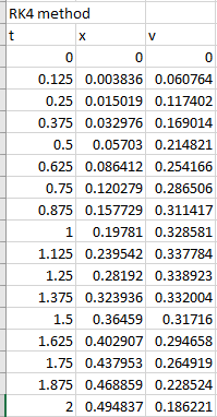
To calculate: The displacement and velocity as a function of time for non-linear system where
Answer to Problem 49P
Solution:
| t | x | v |
| 0 | 0 | 0 |
| 0.125 | 0.003836 | 0.060764 |
| 0.25 | 0.015019 | 0.117402 |
| 0.375 | 0.032976 | 0.169014 |
| 0.5 | 0.05703 | 0.214821 |
| 0.625 | 0.086412 | 0.254166 |
| 0.75 | 0.120279 | 0.286506 |
| 0.875 | 0.157729 | 0.311417 |
| 1 | 0.19781 | 0.328581 |
| 1.125 | 0.239542 | 0.337784 |
| 1.25 | 0.28192 | 0.338923 |
| 1.375 | 0.323936 | 0.332004 |
| 1.5 | 0.36459 | 0.31716 |
| 1.625 | 0.402907 | 0.294658 |
| 1.75 | 0.437953 | 0.264919 |
| 1.875 | 0.468859 | 0.228524 |
| 2 | 0.494837 | 0.186221 |
| 2.125 | 0.515205 | 0.138911 |
| 2.25 | 0.5294 | 0.087637 |
| 2.375 | 0.536996 | 0.033543 |
| 2.5 | 0.537718 | -0.02217 |
| 2.625 | 0.531437 | -0.07829 |
| 2.75 | 0.518177 | -0.13366 |
| 2.875 | 0.498099 | -0.18721 |
| 3 | 0.47149 | -0.23801 |
| 3.125 | 0.438743 | -0.28531 |
| 3.25 | 0.400333 | -0.32852 |
| 3.375 | 0.3568 | -0.36723 |
| 3.5 | 0.308725 | -0.40117 |
| 3.625 | 0.256712 | -0.43023 |
| 3.75 | 0.201374 | -0.45436 |
| 3.875 | 0.143325 | -0.47361 |
| 4 | 0.083172 | -0.48804 |
| 4.125 | 0.021513 | -0.49771 |
| 4.25 | -0.04106 | -0.50268 |
| 4.375 | -0.10396 | -0.50296 |
| 4.5 | -0.1666 | -0.49854 |
| 4.625 | -0.2284 | -0.48938 |
| 4.75 | -0.28875 | -0.47544 |
| 4.875 | -0.34705 | -0.45667 |
| 5 | -0.40271 | -0.43306 |
Explanation of Solution
Given Information:
The dynamic of a forced spring-mass-damper system is given as,
The values,
And,
The initial condition,
Formula used:
The fourth-order RK method for
Where,
Calculation:
Consider the dynamic of a forced spring-mass-damper system,
As
Divide both the sides of above equation by m,
Now, substitute the values
For linear, substitute
Use VBA code for RK4 method as below to solve for x and v,
Code:
Output:
Few data are shown below,
To draw the graph of the above results, follow the steps in excel sheet as given below,
Step 1: Select the cell from A4 to A205 and cell B4 to B205. Then, go to the Insert and select the scatter with smooth lines from the chart.
Step 2: Select the cell from A4 to A205 and cell C4 to C205. Then, go to the Insert and select the scatter with smooth lines from the chart.
Step 3: Select one of the graphs and paste it on another graph to merge the graphs.
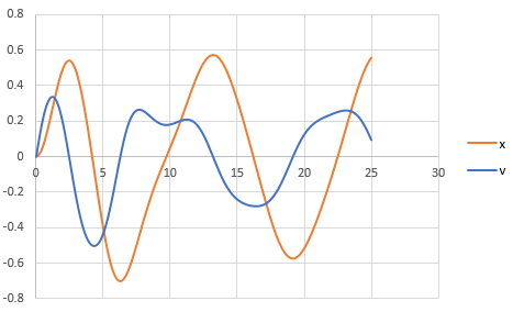
The graph obtained is,
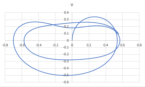
And, to draw the phase plane plot follow the steps as below,
Step 4: Select the column B and column C. Then, go to the Insert and select the scatter with smooth lines from the chart.
The graph obtained is,
Want to see more full solutions like this?
Chapter 28 Solutions
EBK NUMERICAL METHODS FOR ENGINEERS


 Advanced Engineering MathematicsAdvanced MathISBN:9780470458365Author:Erwin KreyszigPublisher:Wiley, John & Sons, Incorporated
 Numerical Methods for EngineersAdvanced MathISBN:9780073397924Author:Steven C. Chapra Dr., Raymond P. CanalePublisher:McGraw-Hill Education
 Introductory Mathematics for Engineering Applicat...Advanced MathISBN:9781118141809Author:Nathan KlingbeilPublisher:WILEY
 Mathematics For Machine TechnologyAdvanced MathISBN:9781337798310Author:Peterson, John.Publisher:Cengage Learning,
