
Videos
The following nonlinear, parasitic ODE was suggested by Hornbeck (1975):
If the initial condition is
(a) Analytically
(b) Using the fourth-order RK method with a constant step size of 0.03125.
(c) Using the MATLAB function ode45.
(d) Using the MATLAB function ode23s.
(e) Using the MATLAB function ode23tb.
Present your results in graphical form.
(a)
To calculate: The analytical solution of the nonlinear, parasitic ordinary differential equation,
Answer to Problem 27P
Solution:
The analytical solution of the differential equation is
Explanation of Solution
Given Information:
A nonlinear, parasitic ordinary differential equation,
Formula used:
The general linear differential equation is,
Calculation:
Consider the nonlinear ordinary differential equation,
Rearrange the above differential equationto get,
Now, compare the above differential equation with the general linear differential equation
Thus,
Now, find the integrating factor (I. F.) as shown below,
Therefore, the solution of the linear differential equation is given as,
Substitute the value of integrating factor (I. F.) in above equation,
Now, integrate the right-hand-side of the above equation,
Solve further, to get
Thus, the solution is
Now, to determine the constant c, use the initial condition
Substitute
Therefore,
Hence, the solution of the differential equation is
(b)
To calculate: Thesolution of the nonlinear, parasitic ordinary differential equation,
Answer to Problem 27P
Solution:
The graph of the solution of the differential equation is,
Explanation of Solution
Given Information:
A nonlinear, parasitic ordinary differential equation,
Calculation:
Consider the nonlinear ordinary differential equation,
The VBA code to solve the above differential equation with fourth-order RK method with a constant step size of 0.03125 is given below,
The output given below is obtained in the Excel after the execution of the above code:
| 4th order RK | ||
| t | y1 | |
| 0 | 0.08 | 0.08 |
| 0.03125 | 0.093476 | 0.093477 |
| 0.0625 | 0.108906 | 0.108906 |
| 0.09375 | 0.126289 | 0.126289 |
| 0.125 | 0.145625 | 0.145625 |
| 0.15625 | 0.166914 | 0.166914 |
| 0.1875 | 0.190156 | 0.190156 |
| 0.21875 | 0.215351 | 0.215352 |
| 0.25 | 0.242499 | 0.2425 |
| 0.28125 | 0.2716 | 0.271602 |
| 0.3125 | 0.302655 | 0.302656 |
| 0.34375 | 0.335662 | 0.335664 |
| 0.375 | 0.370622 | 0.370625 |
| 0.40625 | 0.407536 | 0.407539 |
| 0.4375 | 0.446403 | 0.446406 |
| 0.46875 | 0.487222 | 0.487227 |
| 0.5 | 0.529995 | 0.53 |
| 0.53125 | 0.57472 | 0.574727 |
| 0.5625 | 0.621399 | 0.621406 |
| 0.59375 | 0.670031 | 0.670039 |
| 0.625 | 0.720615 | 0.720625 |
| 0.65625 | 0.773152 | 0.773164 |
| 0.6875 | 0.827642 | 0.827656 |
| 0.71875 | 0.884085 | 0.884102 |
| 0.75 | 0.942481 | 0.9425 |
| 0.78125 | 1.002829 | 1.002852 |
| 0.8125 | 1.06513 | 1.065156 |
| 0.84375 | 1.129383 | 1.129414 |
| 0.875 | 1.195589 | 1.195625 |
| 0.90625 | 1.263747 | 1.263789 |
| 0.9375 | 1.333857 | 1.333906 |
| 0.96875 | 1.405919 | 1.405977 |
| 1 | 1.479932 | 1.48 |
| 1.03125 | 1.555897 | 1.555977 |
| 1.0625 | 1.633814 | 1.633906 |
| 1.09375 | 1.713681 | 1.713789 |
| 1.125 | 1.795498 | 1.795625 |
| 1.15625 | 1.879266 | 1.879414 |
| 1.1875 | 1.964983 | 1.965156 |
| 1.21875 | 2.052649 | 2.052852 |
| 1.25 | 2.142263 | 2.1425 |
| 1.28125 | 2.233824 | 2.234102 |
| 1.3125 | 2.327332 | 2.327656 |
| 1.34375 | 2.422785 | 2.423164 |
| 1.375 | 2.520181 | 2.520625 |
| 1.40625 | 2.61952 | 2.620039 |
| 1.4375 | 2.7208 | 2.721406 |
| 1.46875 | 2.824017 | 2.824727 |
| 1.5 | 2.929171 | 2.93 |
| 1.53125 | 3.036257 | 3.037227 |
| 1.5625 | 3.145273 | 3.146406 |
| 1.59375 | 3.256214 | 3.257539 |
| 1.625 | 3.369075 | 3.370625 |
| 1.65625 | 3.483852 | 3.485664 |
| 1.6875 | 3.600538 | 3.602656 |
| 1.71875 | 3.719125 | 3.721602 |
| 1.75 | 3.839605 | 3.8425 |
| 1.78125 | 3.961966 | 3.965352 |
| 1.8125 | 4.086198 | 4.090156 |
| 1.84375 | 4.212287 | 4.216914 |
| 1.875 | 4.340215 | 4.345625 |
| 1.90625 | 4.469964 | 4.476289 |
| 1.9375 | 4.601512 | 4.608906 |
| 1.96875 | 4.734831 | 4.743477 |
| 2 | 4.869893 | 4.88 |
| 2.03125 | 5.00666 | 5.018477 |
| 2.0625 | 5.145091 | 5.158906 |
| 2.09375 | 5.285137 | 5.301289 |
| 2.125 | 5.426742 | 5.445625 |
| 2.15625 | 5.569837 | 5.591914 |
| 2.1875 | 5.714346 | 5.740156 |
| 2.21875 | 5.860176 | 5.890352 |
| 2.25 | 6.007221 | 6.0425 |
| 2.28125 | 6.155356 | 6.196602 |
| 2.3125 | 6.304436 | 6.352656 |
| 2.34375 | 6.454288 | 6.510664 |
| 2.375 | 6.604715 | 6.670625 |
| 2.40625 | 6.755482 | 6.832539 |
| 2.4375 | 6.906318 | 6.996406 |
| 2.46875 | 7.056903 | 7.162227 |
| 2.5 | 7.206864 | 7.33 |
| 2.53125 | 7.355766 | 7.499727 |
| 2.5625 | 7.503099 | 7.671406 |
| 2.59375 | 7.648268 | 7.845039 |
| 2.625 | 7.790577 | 8.020625 |
| 2.65625 | 7.92921 | 8.198164 |
| 2.6875 | 8.063218 | 8.377656 |
| 2.71875 | 8.191486 | 8.559102 |
| 2.75 | 8.312714 | 8.7425 |
| 2.78125 | 8.425381 | 8.927852 |
| 2.8125 | 8.527709 | 9.115156 |
| 2.84375 | 8.617619 | 9.304414 |
| 2.875 | 8.69268 | 9.495625 |
| 2.90625 | 8.750052 | 9.688789 |
| 2.9375 | 8.786412 | 9.883906 |
| 2.96875 | 8.797877 | 10.08098 |
| 3 | 8.779905 | 10.28 |
| 3.03125 | 8.727189 | 10.48098 |
| 3.0625 | 8.633523 | 10.68391 |
| 3.09375 | 8.491649 | 10.88879 |
| 3.125 | 8.293087 | 11.09563 |
| 3.15625 | 8.027917 | 11.30441 |
| 3.1875 | 7.684546 | 11.51516 |
| 3.21875 | 7.249417 | 11.72785 |
| 3.25 | 6.706683 | 11.9425 |
| 3.28125 | 6.037815 | 12.1591 |
| 3.3125 | 5.221152 | 12.37766 |
| 3.34375 | 4.231369 | 12.59816 |
| 3.375 | 3.038857 | 12.82063 |
| 3.40625 | 1.609002 | 13.04504 |
| 3.4375 | -0.09867 | 13.27141 |
| 3.46875 | -2.13146 | 13.49973 |
| 3.5 | -4.5447 | 13.73 |
| 3.53125 | -7.40305 | 13.96223 |
| 3.5625 | -10.7821 | 14.19641 |
| 3.59375 | -14.7703 | 14.43254 |
| 3.625 | -19.4709 | 14.67063 |
| 3.65625 | -25.0048 | 14.91066 |
| 3.6875 | -31.5132 | 15.15266 |
| 3.71875 | -39.1613 | 15.3966 |
| 3.75 | -48.1421 | 15.6425 |
| 3.78125 | -58.6814 | 15.89035 |
| 3.8125 | -71.043 | 16.14016 |
| 3.84375 | -85.5354 | 16.39191 |
| 3.875 | -102.519 | 16.64563 |
| 3.90625 | -122.417 | 16.90129 |
| 3.9375 | -145.72 | 17.15891 |
| 3.96875 | -173.006 | 17.41848 |
| 4 | -204.949 | 17.68 |
| 4.03125 | -242.336 | 17.94348 |
| 4.0625 | -286.088 | 18.20891 |
| 4.09375 | -337.283 | 18.47629 |
| 4.125 | -397.179 | 18.74563 |
| 4.15625 | -467.248 | 19.01691 |
| 4.1875 | -549.211 | 19.29016 |
| 4.21875 | -645.079 | 19.56535 |
| 4.25 | -757.205 | 19.8425 |
| 4.28125 | -888.338 | 20.1216 |
| 4.3125 | -1041.69 | 20.40266 |
| 4.34375 | -1221.03 | 20.68566 |
| 4.375 | -1430.74 | 20.97063 |
| 4.40625 | -1675.96 | 21.25754 |
| 4.4375 | -1962.71 | 21.54641 |
| 4.46875 | -2297.99 | 21.83723 |
| 4.5 | -2690.02 | 22.13 |
| 4.53125 | -3148.39 | 22.42473 |
| 4.5625 | -3684.34 | 22.72141 |
| 4.59375 | -4310.97 | 23.02004 |
| 4.625 | -5043.62 | 23.32063 |
| 4.65625 | -5900.23 | 23.62316 |
| 4.6875 | -6901.75 | 23.92766 |
| 4.71875 | -8072.7 | 24.2341 |
| 4.75 | -9441.73 | 24.5425 |
| 4.78125 | -11042.3 | 24.85285 |
| 4.8125 | -12913.7 | 25.16516 |
| 4.84375 | -15101.5 | 25.47941 |
| 4.875 | -17659.5 | 25.79563 |
| 4.90625 | -20650.1 | 26.11379 |
| 4.9375 | -24146.4 | 26.43391 |
| 4.96875 | -28234.2 | 26.75598 |
Now, plot the following chart using the data obtained in Excel.
In the above plot, the series1 represent the numerical solution whereas the series2 represent the exact solution.
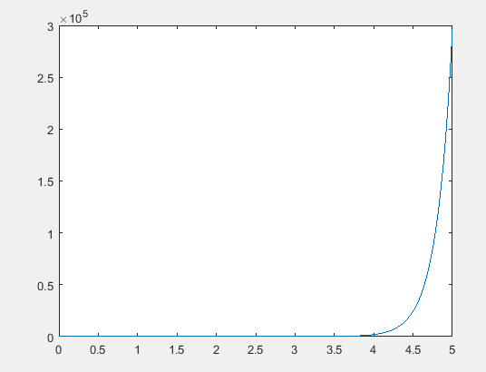
(c)
The solution of the nonlinear, parasitic ordinary differential equation,
Answer to Problem 27P
Solution:
The graph of the solution of the differential equation is,
Explanation of Solution
Given Information:
A nonlinear, parasitic ordinary differential equation,
Consider the nonlinear ordinary differential equation,
Use the MATLAB function
Write the code given below in MATLAB editor window and save it.
function
Now, write the following code in MATLAB command window
Following graph is obtained after the execution of the above MATLAB code.
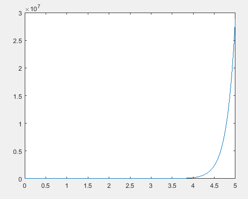
(d)
The solution of the nonlinear, parasitic ordinary differential equation,
Answer to Problem 27P
Solution:
The graph of the solution of the differential equation is,
Explanation of Solution
Given Information:
A nonlinear, parasitic ordinary differential equation,
Consider the nonlinear ordinary differential equation,
Use the MATLAB function
Write the code given below in MATLAB editor window and save it.
function
Now, write the following code in MATLAB command window
Following graph is obtained after the execution of the above MATLAB code.
(e)
The solution of the nonlinear, parasitic ordinary differential equation,
Answer to Problem 27P
Solution:
The graph of the solution of the differential equation is,
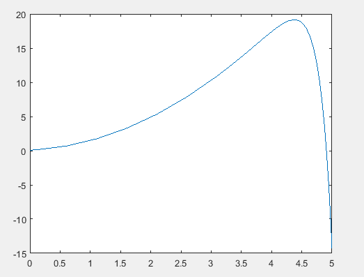
Explanation of Solution
Given Information:
A nonlinear, parasitic ordinary differential equation,
Consider the nonlinear ordinary differential equation,
Use the MATLAB function
Write the code given below in MATLAB editor window and save it.
function
Now, write the following code in MATLAB command window
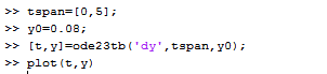
Following graph is obtained after the execution of the above MATLAB code.
Want to see more full solutions like this?
Chapter 27 Solutions
Numerical Methods For Engineers, 7 Ed
Additional Math Textbook Solutions
Basic Technical Mathematics
Advanced Engineering Mathematics
Fundamentals of Differential Equations (9th Edition)
Calculus: Single And Multivariable


- Hello, could I get some help with a Differential Equations problem that involves Eigenvalues and Eigenvectors? The set up is: There are two toy rail cars, Car 1, and Car 2. Car 1 has a mass of 2 kg, and is traveling 3 m/s towards Car 2, which has a mass of 1 kg, and is traveling towards Car 1 at 2 m/s. There is a bumper on the second rail car that engages at the moment the cars hit (connecting Car 1 and Car 2), and does not let go. The bumper acts like a spring with spring constant K = 2 N/m. Car 2 is 7 m from the wall at the time of collision (Car 2 is between Car 1 and the wall). I have attached the work I have done so far, but I'm not understanding how to find x1(t) and x2(t), how we know Car 2 hits the wall (or moves away from it), and at what speed Car 1 travels to stay in place after link-up (given: 1 m/s, but not sure why that is). Thank you in advance.arrow_forwardQuestion 4. Consider the instance F4 || Cmax Wwith no buffer (means jobs are not unload from previous machine until next machine is not available) in front of all machines except M1. Apply NEH Algorithm to minimize the Cmax Jobs 1 2 3 6 М1 17 13 29 23 37 31 М2 25 27 33 31 37 41 M 3 52 14 43 34 25 47 М4 28 31 48 43 18 17arrow_forwardA mechanical system is represented by two masses and three springs, where m, = 12 kg, m, = 22kg, and spring constants k, = k, = k, = 15 N/m, as shown in the following figure. k3 m2 Determine the largest eigenvalue of this mechanical system using the characteristic equation. a. b. Determine the smallest eigenvalue and the corresponding eigenvector using Inverse Power method. Given the initial eigenvector v(0)= (1 1 1). Iterate until | Ar41 - 1x 50.0005.arrow_forward
- Find the Laplace transform of the given function; b iş a real constant. f(t) = cos(bt) Your answer should be an expression in terms of b and s. NOTE: Your answer must be fully simplified. It cannot contain i. L{f(t)}(s) = F(s)arrow_forwardA// Use Implicit Method to solve the temperature distribution of a long thin rod with a length of 9 cm and following values: k = 0.49 cal/(s cm °C), Ax = 3 cm, and At = 0.2 s. At t=0 s, the temperature of the rod is 10°C and the boundary conditions are fixed dT (9,t) 1 °C/cm. Note that the rod for alltimes at 7(0,t) = 80°C and derivative condition dx is aluminum with C = 0.2174 cal/g °C) and p = 2.7 g/cm³. Find the temperature values on the inner grid points and the right boundary for t = 0.4 s.arrow_forwardVerify if the following functions are Linear or not. Support your conclusion with appropriate reason. a) F(x) = b) f(x) =rcos wtarrow_forward
- Q5: Solve the differential equation by using Laplace Transformation method? y" + 2y' + 2y = 5 y(0) = a, y'(0) = b %3Darrow_forward1. Consider the following square matrix A = 9 6 (a) Determine the eigenvalues and eigenvector(s) of A. (b) Find the modal matrix M and diagonalize A through similarity transformation M 'AM. do we get a Jordan form or not? Explain why?arrow_forward04 Find the transfer function of the system shown by Mason's Rule, G₁ G₁ G₂ G3 H₁ G5 H₂ 95 Solve the following inverse transform Laplace transformations. 7s +15 C $²+2 Good luckarrow_forward
 Elements Of ElectromagneticsMechanical EngineeringISBN:9780190698614Author:Sadiku, Matthew N. O.Publisher:Oxford University Press
 Mechanics of Materials (10th Edition)Mechanical EngineeringISBN:9780134319650Author:Russell C. HibbelerPublisher:PEARSON
 Thermodynamics: An Engineering ApproachMechanical EngineeringISBN:9781259822674Author:Yunus A. Cengel Dr., Michael A. BolesPublisher:McGraw-Hill Education
 Control Systems EngineeringMechanical EngineeringISBN:9781118170519Author:Norman S. NisePublisher:WILEY
 Mechanics of Materials (MindTap Course List)Mechanical EngineeringISBN:9781337093347Author:Barry J. Goodno, James M. GerePublisher:Cengage Learning
 Engineering Mechanics: StaticsMechanical EngineeringISBN:9781118807330Author:James L. Meriam, L. G. Kraige, J. N. BoltonPublisher:WILEY