Introduction to Probability and Statistics
14th Edition
ISBN: 9781133103752
Author: Mendenhall, William
Publisher: Cengage Learning
expand_more
expand_more
format_list_bulleted
Concept explainers
Videos
Textbook Question
Chapter 2.7, Problem 2.47E
Mercury Concentration in DolphinsEnvironmental scientists are increasinglyconcerned with the accumulation of toxic elementsin marine mammals and the transfer of such elementsto the animals’ offspring. The striped dolphin (Stenellacoeruleoalba), considered to be a toppredator in the marine food chain, was the subjectof one such study. The mercury concentrations(micrograms/gram) in the livers of 28 maIe stripeddolphins were as follows: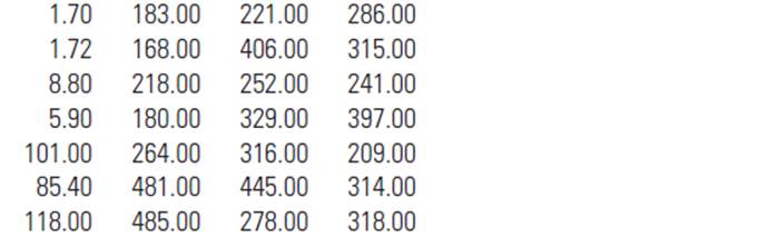
- Calculate the five-number summary for the data.
- Construct a box plot for the data.
- Are there any outliers?
- If you knew that the first four dolphins were allless than 3 years old, while all the others were more than 8 years old, would this information help explainthe difference in the magnitude of those four observations? Explain.
Expert Solution & Answer
Want to see the full answer?
Check out a sample textbook solution
Students have asked these similar questions
A deficiency of the trace element selenium in the diet can negatively impact growth, immunity, muscle and neuromuscular function, and fertility. The introduction of selenium supplements to dairy cows is justified when pastures have low selenium levels. Authors of a research paper supplied the following data on milk selenium concentration (mg/L) for a sample of cows given a selenium supplement (the treatment group) and a control sample given no supplement, both initially and after a 9-day period.
Initial Measurement
Treatment
Control
11.2
9.1
9.6
8.7
10.1
9.7
8.5
10.8
10.3
10.9
10.6
10.6
11.7
10.1
9.7
12.3
10.8
8.8
10.3
10.4
10.4
10.9
11.2
10.4
9.4
11.6
10.6
10.9
10.7
8.4
After 9 Days
Treatment
Control
138.3
9.3
104
8.7
96.4
8.7
89
10.1
88
9.6
103.8
8.6
147.3
10.2
97.1
12.2
172.6
9.3
146.3
9.5
99
8.2
122.3
8.9
103
12.5
117.8
9.1
121.5
93
(a)
Use the given data for the treatment group to determine if there…
A deficiency of the trace element selenium in the diet can negatively impact growth, immunity, muscle and neuromuscular function, and fertility. The introduction of selenium supplements to dairy cows is justified when pastures have low selenium levels. Authors of a research paper supplied the following data on milk selenium concentration (mg/L) for a sample of cows given a selenium supplement (the treatment group) and a control sample given no supplement, both initially and after a 9-day period.
Initial Measurement
Treatment
Control
11.4
9.1
9.6
8.7
10.1
9.7
8.5
10.8
10.2
10.9
10.6
10.6
11.9
10.1
9.9
12.3
10.7
8.8
10.2
10.4
10.3
10.9
11.4
10.4
9.3
11.6
10.6
10.9
10.9
8.3
After 9 Days
Treatment
Control
138.3
9.2
104
8.9
96.4
8.9
89
10.1
88
9.6
103.8
8.6
147.3
10.4
97.1
12.4
172.6
9.2
146.3
9.5
99
8.4
122.3
8.8
103
12.5
117.8
9.1
121.5
93
(a)
Use the given data for the treatment group to determine if…
A deficiency of the trace element selenium in the diet can negatively impact growth, immunity, muscle and neuromuscular function, and fertility. The introduction of selenium supplements to dairy cows is justified when pastures have low selenium levels. Authors of a research paper supplied the following data on milk selenium concentration (mg/L) for a sample of cows given a selenium supplement (the treatment group) and a control sample given no supplement, both initially and after a 9-day period.
Initial Measurement
Treatment
Control
11.3
9.1
9.7
8.7
10.1
9.7
8.5
10.8
10.4
10.9
10.7
10.6
11.8
10.1
9.8
12.3
10.6
8.8
10.4
10.4
10.2
10.9
11.3
10.4
9.2
11.6
10.7
10.9
10.8
8.2
After 9 Days
Treatment
Control
138.3
9.4
104
8.8
96.4
8.8
89
10.1
88
9.7
103.8
8.7
147.3
10.3
97.1
12.3
172.6
9.4
146.3
9.5
99
8.3
122.3
8.9
103
12.5
117.8
9.1
121.5
93
(a)
Use the given data for the treatment group to determine if…
Chapter 2 Solutions
Introduction to Probability and Statistics
Ch. 2.2 - You are given n=5 measurements: 0, 5, 1, 1,3. Draw...Ch. 2.2 - Prob. 2.2ECh. 2.2 - Prob. 2.3ECh. 2.2 - Auto Insurance The cost of automobile insurance...Ch. 2.2 - Prob. 2.5ECh. 2.2 - Prob. 2.6ECh. 2.2 - Prob. 2.7ECh. 2.2 - Prob. 2.8ECh. 2.2 - Prob. 2.9ECh. 2.2 - Prob. 2.10E
Ch. 2.2 - Prob. 2.11ECh. 2.2 - Prob. 2.12ECh. 2.3 - You are given n=5 measurements: 2, 1, 1,3,5. a....Ch. 2.3 - Prob. 2.14ECh. 2.3 - Prob. 2.15ECh. 2.3 - Prob. 2.16ECh. 2.3 - Prob. 2.17ECh. 2.3 - Utility Bills in Southern CaliforniaThe monthly...Ch. 2.5 - Prob. 2.19ECh. 2.5 - Prob. 2.20ECh. 2.5 - A distribution of measurements is relatively...Ch. 2.5 - Prob. 2.22ECh. 2.5 - Prob. 2.23ECh. 2.5 - Packaging Hamburger Meat The data listed here are...Ch. 2.5 - Breathing Rates Is your breathing rate normal?...Ch. 2.5 - Prob. 2.26ECh. 2.5 - Social Security Numbers A group of70 students were...Ch. 2.5 - Prob. 2.28ECh. 2.5 - Prob. 2.29ECh. 2.5 - Prob. 2.30ECh. 2.5 - Timber Tracts To estimate the amount of lumber in...Ch. 2.5 - Prob. 2.32ECh. 2.5 - Prob. 2.33ECh. 2.5 - Prob. 2.34ECh. 2.5 - Prob. 2.35ECh. 2.5 - Prob. 2.36ECh. 2.5 - Prob. 2.37ECh. 2.5 - Prob. 2.38ECh. 2.5 - Prob. 2.39ECh. 2.7 - Prob. 2.40ECh. 2.7 - Find the five-number summary and the IQR forthese...Ch. 2.7 - Given the following data set: 2.3, 1.0, 2.1, 6.5,...Ch. 2.7 - Given the following data set: .23, .30, .35, .41,...Ch. 2.7 - Construct a box plot for these data and...Ch. 2.7 - Construct a box plot for these data and...Ch. 2.7 - If you scored at the 69th percentile on a...Ch. 2.7 - Mercury Concentration in DolphinsEnvironmental...Ch. 2.7 - Hamburger Meat The weights (in pounds) of the 27...Ch. 2.7 - Comparing NFL Quarterbacks How does Aaron Rodgers,...Ch. 2.7 - Presidential Vetoes The set of presidential vetoes...Ch. 2.7 - Survival Times Altman and Bland report the...Ch. 2.7 - Utility Bills in Southern California, again The...Ch. 2.7 - What’s Normal? again Refer to Exercise1.67 and...Ch. 2 - Raisins The number of raisins in each of...Ch. 2 - Prob. 2.55SECh. 2 - Prob. 2.56SECh. 2 - A Recurring IIIness Refer to Exercise 1.26 and...Ch. 2 - Prob. 2.58SECh. 2 - Prob. 2.59SECh. 2 - Tuna Fish, again Refer to Exercise 2.8. Theprices...Ch. 2 - Prob. 2.61SECh. 2 - Chloroform According to the EPA, Chloroform, which...Ch. 2 - Prob. 2.63SECh. 2 - Sleep and the College Student How muchsleep do you...Ch. 2 - Prob. 2.65SECh. 2 - Prob. 2.66SECh. 2 - Polluted Seawater Petroleum pollution in seasand...Ch. 2 - Prob. 2.68SECh. 2 - Prob. 2.69SECh. 2 - Prob. 2.70SECh. 2 - Prob. 2.71SECh. 2 - Prob. 2.72SECh. 2 - Prob. 2.73SECh. 2 - Prob. 2.74SECh. 2 - TV Commercials The mean duration oftelevision...Ch. 2 - Prob. 2.76SECh. 2 - Prob. 2.77SECh. 2 - Prob. 2.78SECh. 2 - Prob. 2.79SECh. 2 - Prob. 2.80SECh. 2 - Prob. 2.81SECh. 2 - Prob. 2.82SECh. 2 - Prob. 2.83SECh. 2 - Prob. 2.84SECh. 2 - Prob. 2.85SE
Knowledge Booster


Learn more about
Need a deep-dive on the concept behind this application? Look no further. Learn more about this topic, statistics and related others by exploring similar questions and additional content below.Similar questions
- Urban Travel Times Population of cities and driving times are related, as shown in the accompanying table, which shows the 1960 population N, in thousands, for several cities, together with the average time T, in minutes, sent by residents driving to work. City Population N Driving time T Los Angeles 6489 16.8 Pittsburgh 1804 12.6 Washington 1808 14.3 Hutchinson 38 6.1 Nashville 347 10.8 Tallahassee 48 7.3 An analysis of these data, along with data from 17 other cities in the United States and Canada, led to a power model of average driving time as a function of population. a Construct a power model of driving time in minutes as a function of population measured in thousands b Is average driving time in Pittsburgh more or less than would be expected from its population? c If you wish to move to a smaller city to reduce your average driving time to work by 25, how much smaller should the city be?arrow_forward4. Medicinal value of plants. Sea buckthorn (Hippophae), a plant that typically grows at high altitudes in Europe and Asia, has been found to have medicinal value. The medicinal properties of berries collected from sea buckthorn were investigated in Academia Journal of Medicinal Plants (Aug. 2013). The following variables were measured for each plant sampled. Identify each as producing quantitative or qualitative data. Species of sea buckthorn (H. rhamnoides, H. gyantsensis, H. neurocarpa, H. tibetana, or H. salicifolia) Altitude of collection location (meters) Total flavonoid content in berries (milligrams per gram) а. b. с.arrow_forwardThe following is data about the hemoglobin concentrations of volunteers collected at sea level and at an altitude of 11000 feet. sea level concentrations = [14.70 , 15.22, 15.28, 16.58, 15.10 , 15.66, 15.91, 14.41, 14.73, 15.09, 15.62, 14.92]11000 feet concentrations = [14.81, 15.68, 15.57, 16.59, 15.21, 15.69, 16.16, 14.68, 15.09, 15.30 , 16.15, 14.76] There are two alternative scenarios about the way the data were obtained. In scenario 1, there are 12 volunteers who lived for a month at sea level, at which time blood was drawn and the data in "sea level concentrations" dataset were obtained. Subsequently, all 12 volunteers were moved to 11000 ft and after a month the data in the "11000 feet concentrations" dataset obtained. There is a one to one correspondence between the numbers in the two datasets, that is the first numbers correspond to volunteer1, the second numbers to volunteer2 etc. In scenario 2, the "sea level concentrations" dataset is a random sample obtained from 12…arrow_forward
- The following is data about the hemoglobin concentrations of volunteers collected at sea level and at an altitude of 11000 feet. sea level concentrations = [14.70 , 15.22, 15.28, 16.58, 15.10 , 15.66, 15.91, 14.41, 14.73, 15.09, 15.62, 14.92]11000 feet concentrations = [14.81, 15.68, 15.57, 16.59, 15.21, 15.69, 16.16, 14.68, 15.09, 15.30 , 16.15, 14.76] There are two alternative scenarios about the way the data were obtained. In scenario 1, there are 12 volunteers who lived for a month at sea level, at which time blood was drawn and the data in "sea level concentrations" dataset were obtained. Subsequently, all 12 volunteers were moved to 11000 ft and after a month the data in the "11000 feet concentrations" dataset obtained. There is a one to one correspondence between the numbers in the two datasets, that is the first numbers correspond to volunteer1, the second numbers to volunteer2 etc. In scenario 2, the "sea level concentrations" dataset is a random sample obtained from 12…arrow_forwardThe following is data about the hemoglobin concentrations of volunteers collected at sea level and at an altitude of 11000 feet. sea level concentrations = [14.70 , 15.22, 15.28, 16.58, 15.10 , 15.66, 15.91, 14.41, 14.73, 15.09, 15.62, 14.92]11000 feet concentrations = [14.81, 15.68, 15.57, 16.59, 15.21, 15.69, 16.16, 14.68, 15.09, 15.30 , 16.15, 14.76] There are two alternative scenarios about the way the data were obtained. In scenario 1, there are 12 volunteers who lived for a month at sea level, at which time blood was drawn and the data in "sea level concentrations" dataset were obtained. Subsequently, all 12 volunteers were moved to 11000 ft and after a month the data in the "11000 feet concentrations" dataset obtained. There is a one to one correspondence between the numbers in the two datasets, that is the first numbers correspond to volunteer1, the second numbers to volunteer2 etc. In scenario 2, the "sea level concentrations" dataset is a random sample obtained from 12…arrow_forwardThe following is data about the hemoglobin concentrations of volunteers collected at sea level and at an altitude of 11000 feet. sea level concentrations = [14.70 , 15.22, 15.28, 16.58, 15.10 , 15.66, 15.91, 14.41, 14.73, 15.09, 15.62, 14.92]11000 feet concentrations = [14.81, 15.68, 15.57, 16.59, 15.21, 15.69, 16.16, 14.68, 15.09, 15.30 , 16.15, 14.76] There are two alternative scenarios about the way the data were obtained. In scenario 1, there are 12 volunteers who lived for a month at sea level, at which time blood was drawn and the data in "sea level concentrations" dataset were obtained. Subsequently, all 12 volunteers were moved to 11000 ft and after a month the data in the "11000 feet concentrations" dataset obtained. There is a one to one correspondence between the numbers in the two datasets, that is the first numbers correspond to volunteer1, the second numbers to volunteer2 etc. In scenario 2, the "sea level concentrations" dataset is a random sample obtained from 12…arrow_forward
- The following is data about the hemoglobin concentrations of volunteers collected at sea level and at an altitude of 11000 feet. sea level concentrations = [14.70 , 15.22, 15.28, 16.58, 15.10 , 15.66, 15.91, 14.41, 14.73, 15.09, 15.62, 14.92]11000 feet concentrations = [14.81, 15.68, 15.57, 16.59, 15.21, 15.69, 16.16, 14.68, 15.09, 15.30 , 16.15, 14.76] There are two alternative scenarios about the way the data were obtained. In scenario 1, there are 12 volunteers who lived for a month at sea level, at which time blood was drawn and the data in "sea level concentrations" dataset were obtained. Subsequently, all 12 volunteers were moved to 11000 ft and after a month the data in the "11000 feet concentrations" dataset obtained. There is a one to one correspondence between the numbers in the two datasets, that is the first numbers correspond to volunteer1, the second numbers to volunteer2 etc. In scenario 2, the "sea level concentrations" dataset is a random sample obtained from 12…arrow_forwardThe following is data about the hemoglobin concentrations of volunteers collected at sea level and at an altitude of 11000 feet. sea level concentrations = [14.70 , 15.22, 15.28, 16.58, 15.10 , 15.66, 15.91, 14.41, 14.73, 15.09, 15.62, 14.92]11000 feet concentrations = [14.81, 15.68, 15.57, 16.59, 15.21, 15.69, 16.16, 14.68, 15.09, 15.30 , 16.15, 14.76] There are two alternative scenarios about the way the data were obtained. In scenario 1, there are 12 volunteers who lived for a month at sea level, at which time blood was drawn and the data in "sea level concentrations" dataset were obtained. Subsequently, all 12 volunteers were moved to 11000 ft and after a month the data in the "11000 feet concentrations" dataset obtained. There is a one to one correspondence between the numbers in the two datasets, that is the first numbers correspond to volunteer1, the second numbers to volunteer2 etc. In scenario 2, the "sea level concentrations" dataset is a random sample obtained from 12…arrow_forwardA cohort study was undertaken to test for association between arteriolosclerosis (hardening of the arterioles) and secondary hypertension. The data were split into 2 groups: subjects who had been treated with nonsteroidal anti-inflammatory drugs (NSAIDS) and those who had not. The stratified data are shown in Table 3: Treated with NSAIDS Exposure Category Secondary Hypertension No Secondary Hypertension Total Not Treated with NSAIDS Exposure Category Secondary Hypertension No Secondary Hypertension Total Table 3 Arteriolosclerosis 46 23 69 Arteriolosclerosis 79 25 104 No Arteriolosclerosis 251 724 975 No Arteriolosclerosis 405 446 851 Total 297 747 1044 Total 484 471 955 Obtain the stratum-specific odds ratios for the 2 groups and the odds ratio for the aggregate data. Comment on the association between arteriolosclerosis and secondary hypertension and the role played by NSAIDS in this association.arrow_forward
- The epidemiological, clinical, and bacteriological aspects of shigellosis were studied in a population of hospitalized children in northern Israel. Shigellosis invades epithelial cells of the colon and causes inflammation a severe cases of diarrhea and dysentery. Below is a table that lists the frequencies of two different species of Shigella: S. sonnei and S. Flexneri between hospitalized and non-hospitalized Jews and Arabs. a) Combine hospitalized and non-hospitalized children, what is the overall prevalence of: sonnei among Jewish children: ____________________________ sonnei among Arab children: ____________________________ Flexneri among Jewish children: ____________________________ Flexneri among Arab children: ____________________________ b) Calculate a 95% confidence interval for the population difference in prevalence of S. Flexneri between hospitalized Jewish children and hospitalized Arab children. Briefly interpret the confidence interval. c) Conduct the appropriate…arrow_forwardIn a study conducted in Italy, 10 patients with hypertriglyceridemia were placed on a low-fat, high-carbohydrate diet. Before the start of the diet, cholesterol and triglyceride measurements were recorded for each subject. Patient Cholesterol Level (mmol/l) Triglyceride level (mmol/l) 1 5.12 2.30 2 6.18 2.54 3 6.77 2.95 4 6.65 3.77 5 6.36 4.18 6 5.90 5.31 7 5.48 5.53 8 6.02 8.83 9 10.34 9.48 10 8.51 14.20A. Use STATA to Calculate the Spearman rank correlation coefficient, rs, for these data. B. Using rs, test the null hypothesis that the population correlation, ρ, equals 0.arrow_forwardIn a study conducted in Italy, 10 patients with hypertriglyceridemia were placed on a low-fat, high-carbohydrate diet. Before the start of the diet, cholesterol and triglyceride measurements were recorded for each subject. Patient Cholesterol Level (mmol/l) Triglyceride level (mmol/l) 1 5.12 2.30 2 6.18 2.54 3 6.77 2.95 4 6.65 3.77 5 6.36 4.18 6 5.90 5.31 7 5.48 5.53 8 6.02 8.83 9 10.34 9.48 10 8.51 14.20 a. Construct a two-way scatter plot for these data. b. Use STATA to calculate Pearson’s Correlation Coefficient for these data. c. Test, α = 0.05, whether or not the population correlation, ρ, equals 0.arrow_forward
arrow_back_ios
SEE MORE QUESTIONS
arrow_forward_ios
Recommended textbooks for you
 Functions and Change: A Modeling Approach to Coll...AlgebraISBN:9781337111348Author:Bruce Crauder, Benny Evans, Alan NoellPublisher:Cengage Learning
 Calculus For The Life SciencesCalculusISBN:9780321964038Author:GREENWELL, Raymond N., RITCHEY, Nathan P., Lial, Margaret L.Publisher:Pearson Addison Wesley,
 Glencoe Algebra 1, Student Edition, 9780079039897...AlgebraISBN:9780079039897Author:CarterPublisher:McGraw Hill
Functions and Change: A Modeling Approach to Coll...
Algebra
ISBN:9781337111348
Author:Bruce Crauder, Benny Evans, Alan Noell
Publisher:Cengage Learning
Calculus For The Life Sciences
Calculus
ISBN:9780321964038
Author:GREENWELL, Raymond N., RITCHEY, Nathan P., Lial, Margaret L.
Publisher:Pearson Addison Wesley,
Glencoe Algebra 1, Student Edition, 9780079039897...
Algebra
ISBN:9780079039897
Author:Carter
Publisher:McGraw Hill
Statistics 4.1 Point Estimators; Author: Dr. Jack L. Jackson II;https://www.youtube.com/watch?v=2MrI0J8XCEE;License: Standard YouTube License, CC-BY
Statistics 101: Point Estimators; Author: Brandon Foltz;https://www.youtube.com/watch?v=4v41z3HwLaM;License: Standard YouTube License, CC-BY
Central limit theorem; Author: 365 Data Science;https://www.youtube.com/watch?v=b5xQmk9veZ4;License: Standard YouTube License, CC-BY
Point Estimate Definition & Example; Author: Prof. Essa;https://www.youtube.com/watch?v=OTVwtvQmSn0;License: Standard Youtube License
Point Estimation; Author: Vamsidhar Ambatipudi;https://www.youtube.com/watch?v=flqhlM2bZWc;License: Standard Youtube License