
Videos
The upward velocity of a rocket can be computed by the following formula:
Where
To calculate: The height of the rocket at
Answer to Problem 46P
Solution:
All the results are summarized in the table below,
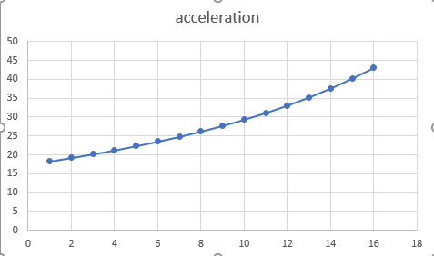
Acceleration graph is shown below.
Explanation of Solution
Given Information:
The formula for the upward velocity of rocket is given as,
Here,
Formula Used:
6-segment Trapezoidal rule.
6-segmentSimpson’s 1/3 rule.
Change of variable formula.
Here,
Error Calculation.
Calculation:
Calculate the upward velocity of the rocket.
Substitute thegiven values in equation(1),
Apply 6-segment Trapezoidal rule for
Here,
Substitute
Expand the above terms.
Calculate
Substitute
Calculate
Substitute
Calculate
Substitute
Similarly, calculate all the function values.
Substitute above values in equation(3),
The formula for 6-segment Simpson’s 1/3 rule,
Substitute the function values from above,
The given velocity Integral is,
Change of variable before integrating the function,
And
Here,
Substitute the values of
Substitute the values of
Thus, the transformed function is,
Apply Six-Point Gauss Quadrature formula.
Calculate
Substitute
Calculate
Substitute
Similarly, calculate all function values.
Substitute the values in Six-Point Gauss Quadrature formula.
Apply Romberg Integration.
Choose
Substitute value from above and calculate
Choose
Substitute values from above and calculate
Choose
Substitute values from above and calculate
Choose
Substitute values from above and calculate
Substitute values from above and calculate
Calculate the approximate error,
Substitute values from above.
Substitute values from above and calculate
Substitute values from above and calculate
Substitute values from above and calculate
Calculate the approximate error,
Substitute values from above,
Substitute values from above and calculate
Substitute values from above and calculate
Calculate the approximate error as,
Substitute values from above.
All above calculated results are summarized in the table below,
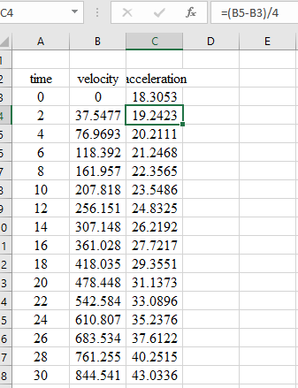
UseNumerical differentiation to calculate acceleration as a function of time.
Apply finite-divided differences for
Apply centred differences to calculate the intermediate values,
Similarly, calculate all intermediate values of acceleration.
Apply backward difference for the last value at t = 30 s,
All of the results are displayed in the following table and graph,
Select the time and acceleration column and go to insert chart and scattered chart. The graph of acceleration verses time is plotted as follows:
Want to see more full solutions like this?
Chapter 24 Solutions
EBK NUMERICAL METHODS FOR ENGINEERS


- . I am planning to perform some volume-flow rate measurements in the Fluid Mechanics Laboratory. For this, I need a volumetric measuring tank (graduated cylinder) and a stopwatch. I considered the volume of the measured tank as 15 gallons and a stopwatch with reaction time as 1/10th of a second (though resolution of 1/1000th of a second). What is the volume flow rate if it takes 5 minutes to fill a 15-gallon of tank? Determine the smallest division to be on the tank in order to estimate the volume flow rate within an accuracy of ± 0.05 gpm.arrow_forwardThe elevations of the ski jumping hill shown below are as follows: hA = 37 mhB = 2.4 mhC = 5.5 m If the velocity of a ski jumper is measured to be 25.3 m/s at position B, what will be the launch velocity (in m/s) at position C [round your final answer to one decimal place]?arrow_forwardMechanical Engineering The following table shows the kinetic energy and potential energy according to the speed of an object descending along a frictionless rain surface. What is the potential energy when the speed is 3/2v ? (It satisfies energy conservation) velocity kinetic energy 1500J potential energy V 3/2 * v 2v 1. 1400 J 2. 1000 J 3. 800 J 4. 600 J Please solve step by step. Thanks in advance! 1600 Jarrow_forward
- Ql: The viscosity in industrial measurement continue to use the CGS system of Lunits, since centimeters and grams vield convenient numbers for many fluids. The absolute viscosity () unit is the poise, I poise = 1 gtem. s). The kinematic viscosity (v) unit is the stohes, I stokes = 1 em /s. Water at 20C has u = 001 poise and also V= 0.01 stokes. Express these resalts in (a) SI and (h) BG tanits.arrow_forwardThe friction force F on a smooth sphere falling in water depends on the sphere speed V, the sphere density ρ_s and diameter D_s, the density ρ and dynamic viscosity μ of the water, gravitational acceleration g. Choose the correct repeating variables. sphere diameter, dynamic viscosity, gravitational acceleration density, gravitational acceleration, dynamic viscosity friction force, gravitational acceleration, density density, sphere speed, sphere diameter friction force, sphere speed, sphere diameterarrow_forwardA snowboarder’s velocity is tracked by a pulse-laser velocimeter as she descends the slope. These velocity data are stored and analyzed via an embedded curve fitting procedure to determine a velocity function of v(t) = 1.5t2 + 2t + 2 (t is time in seconds and v is velocity in ft/s). At time equal 0, position (x) is zero. Find her position (e.g., distance traveled), velocity and acceleration formulations and values of each when time equals 15 seconds. Clearly write the formulas before finding respective values at t = 15 seconds!arrow_forward
- As we explained in earlier chapters, the air resistance to the motion of a vehicle is something important that engineers investigate. The drag force acting on a car is determined experimentally by placing the car in a wind tunnel. The air speed inside the tunnel is changed, and the drag force acting on the car is measured. For a given car, the experimental data generally is represented by a single coefficient that is called drag coefficient. It is defined by the following relationship: F, where air resistance for a car that has a listed C, = drag coefficient (unitless) measured drag force (N) drag coefficient of 0.4 and width of 190 cm and height of 145 cm. Vary the air speed in the range of 15 m/sarrow_forwardIn medical literatures, local blood perfusion rate is typically presented as xx ml/(min 100g tissue), in another word, it represents xx ml of blood supplied to a tissue mass of 100 g per minute to satisfy its nutritional needs. As we learned from the course lectures, the local blood perfusion rate appearing in the Pennes bioheat equation is in a unit of 1/s, or can be interpreted as xx ml of blood supplied to a tissue volume of 1 ml per second. The following lists the blood perfusion rates in various organs or structures in a human body from medical textbooks: brain (50 ml/(min 100g tissue)), kidney (35 ml/(min 100g tissue)), and muscle at rest (3 ml/(min 100g tissue)). Please convert the above local blood perfusion rates into values with the unit of 1/s, therefore, they can be used in the Pennes bioheat equation. The tissue density in a human body is 1050 kg/m³.arrow_forwardQ1/ The figure below shows such an LSPB trajectory, where the maximum velocity V 60 deg/sec. In this case, the times are given as t.= 5 sec and t 30 sec. In addition, the joint angles in beginning and the ending q=20 deg and qf = 70 deg , respectively. For these required data , determine the following : 1- The position function and its profile. 2- The velocity function and its profile. 3- The acceleration function and its profile. 4- The function of jerk variable and what is the nature of jerk? 5- The position, velocity, and acceleration at tm-13 sec. te tm ty te ty tarrow_forwardQ1. The image below shows an example of "absolute dependent motion analysis", where the motions of two objects depend on each other, and the goal is to find the relations in their motions (i.e., in their positions, velocities, and accelerations). Please put the suggested steps of analysis in the correct order. VA A B VB Differentiate the entire equation with respect to time, and extract the relation in velocities. Repeat for acceleration if needed. Set up a coordinate (s) along the direction of motion from a fixed point (O) or a fixed datum line. Represent the positions of the objects respectively. In some cases intermediate objects need to be considered too and their positions need to be represented as well. Recognize the constant length(s) and find the depending geometric relations between the position variables.arrow_forwardYou are designing a spherical tank to hold water for a small village. The volume of liquid it can hold can be computed as V = nh?(3R=h) %3D where V = volume [m³], h = depth of water in tank [m], and R = the tank radius [m]. Use Newton Raphson method with 1 iterations to find the relative percentage error in height calculation (e = 100|(hi+1 – hi)/h;) for storing 20 m³ of water with 10 m diameter-tank. Take T = 3.1416 and initial guess for h=R. %3D %3D Choices 61.5737 60.3422 30.7869 92.3606 Submit I Attempts 1 2 |arrow_forwardThe friction in flows through the pipe is defined by a dimensionless number called the fanning friction factor (f). The Fanning friction factor is represented by another dimensionless number, the Reynolds number (Re).It depends on the diameter of the pipe and some parameters related to the fluid. An equation that can predict f given the Reynolds number is given as follows. If Re =4000, e/D=0.01 in this equation, find the value of f using the Simple Iteration method by taking f0=0.1 as the initial value for the solution (ԑ=0.0001)arrow_forwardarrow_back_iosSEE MORE QUESTIONSarrow_forward_ios
 Elements Of ElectromagneticsMechanical EngineeringISBN:9780190698614Author:Sadiku, Matthew N. O.Publisher:Oxford University Press
 Mechanics of Materials (10th Edition)Mechanical EngineeringISBN:9780134319650Author:Russell C. HibbelerPublisher:PEARSON
 Thermodynamics: An Engineering ApproachMechanical EngineeringISBN:9781259822674Author:Yunus A. Cengel Dr., Michael A. BolesPublisher:McGraw-Hill Education
 Control Systems EngineeringMechanical EngineeringISBN:9781118170519Author:Norman S. NisePublisher:WILEY
 Mechanics of Materials (MindTap Course List)Mechanical EngineeringISBN:9781337093347Author:Barry J. Goodno, James M. GerePublisher:Cengage Learning
 Engineering Mechanics: StaticsMechanical EngineeringISBN:9781118807330Author:James L. Meriam, L. G. Kraige, J. N. BoltonPublisher:WILEY