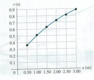
DATA In your physics lab you release a small glider from rest at various points on a long, frictionless air track that is inclined at an angle θ above the horizontal. With an electronic photocell, you measure the time t it takes the glider to slide a distance x from the release point to the bottom of the track. Your measurements are given in Fig. P2.84 , which shows a Figure P2.84 second-order polynomial (quadratic) fit to the plotted data. You are asked to find the glider’s acceleration, which is assumed to be constant. There is some error in each measurement, so instead of using a single set of x and t values, you can be more accurate if you use graphical methods and obtain your measured value of the acceleration from the graph, (a) How can you re-graph the data so that the data points fall close to a straight line? ( Hint: You might want to plot x or t , or both, raised to some power.) (b) Construct the graph you described in part (a) and find the equation for the straight line that is the best fit to the data points, (c) Use the straight-line fit from part (b) to calculate the acceleration of the glider, (d) The glider is released at a distance x = 1.35 m from the bottom of the track. Use the acceleration value you obtained in part (c) to calculate the speed of the glider when it reaches the bottom of the track.
DATA In your physics lab you release a small glider from rest at various points on a long, frictionless air track that is inclined at an angle θ above the horizontal. With an electronic photocell, you measure the time t it takes the glider to slide a distance x from the release point to the bottom of the track. Your measurements are given in Fig. P2.84 , which shows a Figure P2.84 second-order polynomial (quadratic) fit to the plotted data. You are asked to find the glider’s acceleration, which is assumed to be constant. There is some error in each measurement, so instead of using a single set of x and t values, you can be more accurate if you use graphical methods and obtain your measured value of the acceleration from the graph, (a) How can you re-graph the data so that the data points fall close to a straight line? ( Hint: You might want to plot x or t , or both, raised to some power.) (b) Construct the graph you described in part (a) and find the equation for the straight line that is the best fit to the data points, (c) Use the straight-line fit from part (b) to calculate the acceleration of the glider, (d) The glider is released at a distance x = 1.35 m from the bottom of the track. Use the acceleration value you obtained in part (c) to calculate the speed of the glider when it reaches the bottom of the track.
DATA In your physics lab you release a small glider from rest at various points on a long, frictionless air track that is inclined at an angle θ above the horizontal. With an electronic photocell, you measure the time t it takes the glider to slide a distance x from the release point to the bottom of the track. Your measurements are given in Fig. P2.84, which shows a
Figure P2.84
second-order polynomial (quadratic) fit to the plotted data. You are asked to find the glider’s acceleration, which is assumed to be constant. There is some error in each measurement, so instead of using a single set of x and t values, you can be more accurate if you use graphical methods and obtain your measured value of the acceleration from the graph, (a) How can you re-graph the data so that the data points fall close to a straight line? (Hint: You might want to plot x or t, or both, raised to some power.) (b) Construct the graph you described in part (a) and find the equation for the straight line that is the best fit to the data points, (c) Use the straight-line fit from part (b) to calculate the acceleration of the glider, (d) The glider is released at a distance x = 1.35 m from the bottom of the track. Use the acceleration value you obtained in part (c) to calculate the speed of the glider when it reaches the bottom of the track.
You hopefully used g=9.8 m/s2 (or thereabouts). That is the gravitational acceleration near the earth's surface. if you rise high above the earth, the gravitational acceleration decreases. Specifically, the gravitational acceleration is inversely proportional to the square of the distance from the earth's center.
Equivalently, if you multiply the acceleration by the distance from the earth's center, you should get the same number for all heights.
For this problem, take the radius of the earth as 3,902 miles, and calculate the gravitational acceleration of a satellite in low orbit, 182 miles above the surface.
A space shuttle lands on a distant planet where the gravitational acceleration is 2.0 ( We do not know thelocal units of length and time , but they are consistent throughout the problem). The shuttle coasts along aleve, frictionless plane with a speed of 6.0. It then coasts up a frictionless ramp of height 5.0 and angle 0f 30°.After a brief ballistic flight, it lands a distance S from the ramp. Solve for S in local units of length. Assume theshuttle is small compared to the local length unit and that all atmospheric effects are negligible. Use x and y components.
In the vertical jump, an Kobe Bryant starts from a crouch and jumps upward to reach as high as possible. Even the best athletes spend little more than 1.00 s in the air (their "hang time"). Treat Kobe as a particle and let ymax be his maximum height above the floor. Note: this isn't the entire story since Kobe can twist and curl up in the air, but then we can no longer treat him as a particle.
Hint: Find v0 to reach y_max in terms of g and y_max and recall the velocity at y_max is zero. Then find v1 to reach y_max/2 with the same kinematic equation. The time to reach y_max is obtained from v0=g (t), and the time to reach y_max/2 is given by v1-v0= -g(t1). Now, t1 is the time to reach y_max/2, and the quantity t-t1 is the time to go from y_max/2 to y_max. You want the ratio of (t-t1)/t1
Note from Asker: I am generally confused on how to manipulate the formulas, so if you could show every step that would be great, Thank You.
Part A
Part complete
To explain why…
Chapter 2 Solutions
University Physics with Modern Physics (14th Edition)
Need a deep-dive on the concept behind this application? Look no further. Learn more about this topic, physics and related others by exploring similar questions and additional content below.


 Principles of Physics: A Calculus-Based TextPhysicsISBN:9781133104261Author:Raymond A. Serway, John W. JewettPublisher:Cengage Learning