Theory and Design for Mechanical Measurements
6th Edition
ISBN: 9781118881279
Author: Richard S. Figliola, Donald E. Beasley
Publisher: WILEY
expand_more
expand_more
format_list_bulleted
Concept explainers
Videos
Textbook Question
Chapter 2, Problem 2.20P
Find the Fourier series of the function shown in Figure 2.24, assuming the function has a period of 2k. Plot an accurate graph of the first three partial sums of the resulting Fourier series.
Figure 2.24 Function to be expanded in a Fourier series in Problem 2.20

| yW, | |
| 11 1 | — |
| -ITIT | 7T7T |
| 2 -1 | 2 |
Expert Solution & Answer
Want to see the full answer?
Check out a sample textbook solution
Students have asked these similar questions
Compute the Laplace Transforms of the following time domain functions from the Laplace
Transformation definition
a) f(1) =r"
b) f(t) =tcos(wt)
Solve the inverse kinematic problem for the following 6 DOF robot, using the method ofkinematic decouplingif it is known that its Denavit-Hartenberg parameters are as shown in the table inthe table
MA
Figure (2)
3- The time response of a liner spring-mass-damper system with the mass of (m), the stiffness coefficient of (k), and
a dampirg constant of (c) is given below in figure (2) with a set of coordinates marked by fillec circles. x(t) is in
meters, it is in seconds. Indicate the units of all quantities involved in your solutions when calculate
0
-1-
(0.53, 1.78)
(0,0.8)
2
(2.1,-1.3)
(3.7,0.9)
L
4
(5.3,-0.7)
-
The damping ratio of the system.
Its natural frequency w., damping corstart c, and stiffness coefficient k; for (m-1.25 kg).
III- The amplitude of the motion if the phase angle is given as (0.4 rad).
IV. Its initial conditions.
(6.86, 0.5)
10
t[sec]
Chapter 2 Solutions
Theory and Design for Mechanical Measurements
Ch. 2 - Prob. 2.1PCh. 2 - Prob. 2.2PCh. 2 - Research and describe the importance of...Ch. 2 - Research and describe the importance of data...Ch. 2 - Determine the average and rms values for the func...Ch. 2 - Prob. 2.6PCh. 2 - Prob. 2.9PCh. 2 - Prob. 2.10PCh. 2 - Prob. 2.11PCh. 2 - Prob. 2.12P
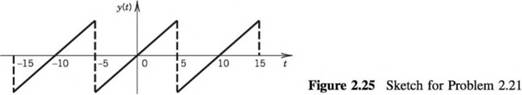
Ch. 2 - Express the function y(t) = 4 sin 2xt + 15 cos...Ch. 2 - Prob. 2.14PCh. 2 - The Fourier series that formed the result for...Ch. 2 - The nth partial sum of a Fourier series is defined...Ch. 2 - For the Fourier series given by where t is time in...Ch. 2 - Determine the Fourier series for the function y(t)...Ch. 2 - Show that y(t) = f2(—jc < t < k), y(t + 2k) = y(t)...Ch. 2 - Find the Fourier series of the function shown in...Ch. 2 - Determine the Fourier series for the function y(t)...Ch. 2 - Determine the Fourier series that represents the...Ch. 2 - Consider the triangle wave shown in Figure 2.26 as...Ch. 2 - Prob. 2.24PCh. 2 - A particle executes linear harmonic motion around...Ch. 2 - Define the following characteristics of signals:...Ch. 2 - Construct an amplitude spectrum plot for the...Ch. 2 - Prob. 2.28PCh. 2 - Sketch representative waveforms of the following...Ch. 2 - Represent the function e(t) = 5 sin 31 At + 2 sin...Ch. 2 - Repeat Problem 2.30 using a data set of 256 num...Ch. 2 - A particular strain sensor is mounted to an...Ch. 2 - Prob. 2.33PCh. 2 - Prob. 2.34PCh. 2 - Consider the upward flow of water and air in a...Ch. 2 - Prob. 2.37PCh. 2 - Prob. 2.38PCh. 2 - For the even-functioned triangle wave signal...Ch. 2 - Prob. 2.40P
Knowledge Booster


Learn more about
Need a deep-dive on the concept behind this application? Look no further. Learn more about this topic, mechanical-engineering and related others by exploring similar questions and additional content below.Similar questions
- 1) Consider the baseband pulse x(1) = n(2) = 11 a) Derive the complex ambiguity function for x(t) and compare your result with the one obtained in class. b) Use MATLAB to compute the complex ambiguity function and compare it to part (a). c) Now, consider the pulse x(t) = sinc(Bt) i) Derive the complex ambiguity function for x(t) and compare to the ambiguity function of the rect pulse. Make your observations. ii) Plot the ambiguity function using the mesh function and using the contour function. iii) Use MATLAB to compute the complex ambiguity function and compare it to part (ii).arrow_forwardsole using laplace transforms Do not answer in image formatarrow_forwardFind the local maximum and minimum values and saddle point(s) of the function. You are encouraged to use a calculator or computer to graph the function with a domain and viewpoint that reveals all the important aspects of the function. (Enter your answers as comma-separated lists. If an answer does not exist, enter DNE.) f(x, y) = 9 sin(x) sin(y), −? < x < ?, −? < y < ? local maximum value(s) local minimum value(s) saddle point(s) (x, y) =arrow_forward
- Obtain the Fourier series expansion for the following function 0arrow_forwardnk int m The spring-mass-system shown in the figure has the following parameters: spring constant k = 4 N/m; mass m 6 %3D kg and the constant n = 1.6. M is the corresponding mass-matrix of the system. V1 and V2 are the eigenvectors associated with the smallest and largest natural frequencies of the system, respectively. If V,TV, = 1 and V2 V2 = 1, then what is value of V,™MV2 (in kg)? Answer:arrow_forwardMy question and answer is in the image. Can you please check my work? A 2 kg mass is attached to a spring with spring constant 50 N/m. The mass is driven by an external force equal tof(t) = 2 sin(5t). The mass is initially released from rest from a point 1 m below the equilibrium position. (Use theconvention that displacements measured below the equilibrium position are positive.)(a) Write the initial-value problem which describes the position of the mass. 2y"+50y=2cos(5t) (b) Find the solution to your initial-value problem from part (a). (1+(1/2)tcos(t))cos(5t)-(1/2)tcos(t) (c) Circle the letter of the graph below that could correspond to the solution. B (d) What is the name for the phenomena this system displays? Resonancearrow_forwardProblem 4-1: During a step function calibration, a first-order instrument is exposed to a step change of 100 units. If after 1.2 s the instrument indicates 80 units, estimate the instrument time constant. Estimate the error in the indicated value after 1.5 s. For this instrument, y (0) = 0 units; K = 1 unit/unit.arrow_forwardTo create AutoCAD Q: Use the principle of the geometric model shown in the following figure? R8 16 22 50 015 50 425 40 80 20 rarrow_forward3. Use the second method of frame assignment, and find the Jacobian of the following robot using the velocity propagation method (Ignore all theta related offsets): 03 02 L2 01 Please answer the question precisely and completely to use the second method of frame assignment to find the D-H table [alpha (i-1) , a (i-1) , d (i) , theta (i)], and find the jacobian matrix using the velocity propagation methodarrow_forwardThe one-dimensional harmonic oscillator has the Lagrangian L = mx˙2 − kx2/2. Suppose you did not know the solution of the motion, but realized that the motion must be periodic and therefore could be described by a Fourier series of the form x(t) =∑j=0 aj cos jωt, (taking t = 0 at a turning point) where ω is the (unknown) angular frequency of the motion. This representation for x(t) defines many_parameter path for the system point in configuration space. Consider the action integral I for two points t1 and t2 separated by the period T = 2π/ω. Show that with this form for the system path, I is an extremum for nonvanishing x only if aj = 0, for j ≠ 1, and only if ω2 = k/m.arrow_forwardQ5. For a point at distance 50 m and angle 450 to the axis which of the following statements are correct? Consider an infinite baffled piston of radius 5 cm driven at 2 kHz in air with velocity 10 m/s. You may choose multiple options. a. The constant term is given by 515.03 b. The distance dependent term is given by e-jk50/50 c. The directivity term is given by j1(Ka sin 450)/sin 450 d. There is no time dependent term.arrow_forward1- According to the system shown below, determine nodal displacements at node number 1 through 5 in meter. (All details of solution steps should be mentioned) k-80 lb/in kg 120 lb/in 100 lbs. HIH k₁-60 lb/in 180 lb/in ky- 50 lb/in 80 lbs. www k₂= 150 lb/inarrow_forwardarrow_back_iosSEE MORE QUESTIONSarrow_forward_ios
Recommended textbooks for you
 Elements Of ElectromagneticsMechanical EngineeringISBN:9780190698614Author:Sadiku, Matthew N. O.Publisher:Oxford University Press
 Mechanics of Materials (10th Edition)Mechanical EngineeringISBN:9780134319650Author:Russell C. HibbelerPublisher:PEARSON
 Thermodynamics: An Engineering ApproachMechanical EngineeringISBN:9781259822674Author:Yunus A. Cengel Dr., Michael A. BolesPublisher:McGraw-Hill Education
 Control Systems EngineeringMechanical EngineeringISBN:9781118170519Author:Norman S. NisePublisher:WILEY
 Mechanics of Materials (MindTap Course List)Mechanical EngineeringISBN:9781337093347Author:Barry J. Goodno, James M. GerePublisher:Cengage Learning
 Engineering Mechanics: StaticsMechanical EngineeringISBN:9781118807330Author:James L. Meriam, L. G. Kraige, J. N. BoltonPublisher:WILEY
Elements Of Electromagnetics
Mechanical Engineering
ISBN:9780190698614
Author:Sadiku, Matthew N. O.
Publisher:Oxford University Press
Mechanics of Materials (10th Edition)
Mechanical Engineering
ISBN:9780134319650
Author:Russell C. Hibbeler
Publisher:PEARSON
Thermodynamics: An Engineering Approach
Mechanical Engineering
ISBN:9781259822674
Author:Yunus A. Cengel Dr., Michael A. Boles
Publisher:McGraw-Hill Education
Control Systems Engineering
Mechanical Engineering
ISBN:9781118170519
Author:Norman S. Nise
Publisher:WILEY
Mechanics of Materials (MindTap Course List)
Mechanical Engineering
ISBN:9781337093347
Author:Barry J. Goodno, James M. Gere
Publisher:Cengage Learning
Engineering Mechanics: Statics
Mechanical Engineering
ISBN:9781118807330
Author:James L. Meriam, L. G. Kraige, J. N. Bolton
Publisher:WILEY
Dynamics - Lesson 1: Introduction and Constant Acceleration Equations; Author: Jeff Hanson;https://www.youtube.com/watch?v=7aMiZ3b0Ieg;License: Standard YouTube License, CC-BY