
Videos
Use a continuous Fourier series to approximate the sawtooth wave in Fig. P19.4. Plot the first three terms along with the summation.
FIGURE P19.4
A sawtooth wave.
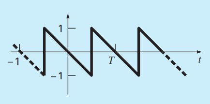
To calculate: The Fourier series expansion to approximate the sawtooth wave, as shown in the following figure,
Plot the first three terms along with the summation.
Answer to Problem 4P
Solution:
The Fourier series of the sawtooth curve is
Explanation of Solution
Given Information: The sawtooth wave shown as,
Formula used:
Consider
And the coefficients are defined by,
Calculation:
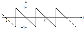
Consider the sawtooth wave as shown in the following figure,
Therefore, the sawtooth wave is a periodic function
;
Therefore, the sawtooth wave,
Therefore, the Fourier series expansion of the function
Here, the coefficients are defined by,
Now, find
Consider,
Thus,
Therefore,
Now, find
Consider,
Thus,
Further,
Therefore,
Therefore, the coefficients of the Fourier series expansions are,
Therefore, the Fourier series expansion defines
Hence,
Graph:
To plot the given sawtooth curve and the approximated Fourier series consider the period,
Therefore, the periodic sawtooth curve is expressed as,
And, the corresponding Fourier series is,
Hence,
Use the following MATLAB code to plot the first three terms along with the summation.
Execute the above code to obtain the plot as,
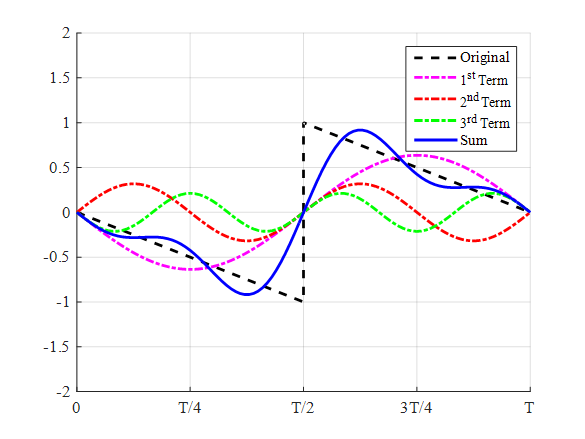
Interpretation: The above plot shows the comparison between the variation in the first three terms of the series along with the variation in summation.
Want to see more full solutions like this?
Chapter 19 Solutions
EBK NUMERICAL METHODS FOR ENGINEERS


- If f (x) is a probability density function then what is the value of (Apr. 2016)arrow_forwardConsider the Exponential Weighted Moving Average that is used to estimate the Round Trip Time (RTT) of a TCP segment. The formula is: EstimatedRTT = (1 - A) * EstimatedRTT + A * SampleRTT Which of the following values of A gives the greatest weight to the most recent samples of round trip times? a. A = 0.25 O b. A = 0.8 О с. А%3D 0.5arrow_forwardIn this exercise we show that in the general case, exact recovery of a linear compression scheme is impossible. a. Let A ∈ Rn,d be anarbitrary compression matrix where n ≤ d−1. Show that there exists u,v ∈ Rd,u= v, such that Au = Av. Hint: Show that there exists u= 0,v = 0 such that Au = Av = 0. Hint: Consider using the rank-nullity theorem. b. Conclude that exact recovery of a linear compression scheme is impossible.arrow_forward
- Please choose the correct dependency relationship. (only one answer is correct) Choose from the following: (A) Clearance (CL) depends on elimination rate constant (k) and volume of distribution (V) (B) Volume of distribution (V) depends on clearance (CL) and elimination rate constant (k) (C) Eliminate rate constant (k) depends on clearance (CL) and volume of distribution (V)arrow_forward立 Bb Slide 1 X 2 28010712 plackboardcdn.com/5c082fb7a0cdb/28010712?X-Blackboard-Expiration3D1645034400000&X-Blackboard-Signature=D06jX8mbU.. LE Seneca Virtual Com... 乙/ L %001 Problem set # 4 Chapter 5 1) A reservoir of water is drained by a 254mm diameter, square-edge orifice with center elevation 88.12m that flows directly into a stream with water surface at elevation 89.49m. The elevation of the reservoir surface is 90.48m. Find the flow through the orifice. 2) A 150-mm- diameter, square-edge orifice convey flow from a reservoir with water level at elevation 79.25m. the center of the orifice is at elevațion 66.10 m. Find the discharge for the free flow. 3) In problem 2 if the tail water is at elevation 71.98m, what is the discharge? 4) Find the discharge over a 90° V-notch weir if the head is 190.5mm. 5) Using the diagram below, find the discharge over the rectangular, sharp-crest weir Elev 37.00 Crest elev. 36.58 Channel inv. 36.12 O 7°C Cloudy ョ ((Dツ hp duarrow_forwardthe same answer as found above. Tutorial Problems No. 2.2 1. Find the ammeter current in Fig. 2.57 by using loop analysis. [1/7 A] (Network Theory Indore Univ. 1981) 10 IK a 10 in 2K 10 10 10K IOK 10 4V 2K 100 V 10 T50 V 10 VT IK 10 Fig. 2.59 Fig. 2.58 Fig. 2.57arrow_forward
- Q2.The numerical solution of the Falknar-Scan Equation f' 0.0 0.0000000 0.000000 f" 0.363600 f + ff + B[1- (f )’]= 0 0.2 0.0093914 0.093905 0.4 0.0375492 0.187605 0.6 0.0843856 0.280575 0.355306 0.327254 0.301734 0.291190 about a plate with pressure gradient are given in Table. Eree stream velocity of air is. 10 m/s. 0.8 0.1496745 0.371963 1.0 0.2329900 0.460632 1.2 0.3336572 0.545246 0.284379 0.270565 Calculate: 1.4 0.4507234 0.624386 0.269692 1.6 0.5829560 0.696699 1.8 0.7288718 0.761057 2.0 0.8867962 0.766694 0.252487 0.240445 a) Boundary laver thickness, 8(x), dispalecement thickness &*(x) and the 0.225669 local friction coefficient. C (x). b) Drag force acting on the plate with 80 in length and 40 cm in width 2.2 1.0549463 0.793303 2.4 1.2315267 0.811065 0.210580 0.167561 2.6 1.4148231 0.830601 0.128613 Note: The density and viscosity of air is 1.12 kg/m and 1.56x10-s m²/s respectively. f' =u/U 2.8 1.6032823 0.852875 3.0 1.7955666 0.879054 0.095114 0.067711 0.046370 3.2 1.9905796…arrow_forwardFourier Methods Questionarrow_forward. Suppose that a wind turbine with a blade length 40 m and power coefficient of 0.27 installed on shore. The air density is 1.2 kg/m'. In a certain day the wind speed was about 13 m/s in the first 8 hours of that day. Then it dropped to 8.5 m/s for the next 10 hours and finally became 7 m/s. Calculate the followings 1) The wind power in each time period of that day. 2) The power generated in each time period of that day. 3) The maximum theoretical generated power in each time period of that day. 4) What is the approximate cost of power generated in this day?arrow_forward
- explains how the two methods of parameter estimation, namely the method of parameter estimation and the method of moments and percentile matching, are used to fit distributions to data for actuarial calculations.arrow_forwardFor the following RRR manipulator and the matrix showing its forward kinematics LA C123 -8123 0.0 c1 +l2C12 0.0 81 +12812 $123 0.0 C123 0.0 %3D 1.0 0.0 1 Using inverse kinamatics and the quick check methods prove that For 0, = 90°, 02 = 0° x = 0 y = Li+ L2arrow_forwardP7.3 A geared DC motor has a built-in incremental encoder that is connected to the motor side. The encoder disk has 1250 lines, and the gear ratio is 9:1. Determine the angular resolution of this encoder, assuming that the encoder is operated in quadrature mode.arrow_forward
 Elements Of ElectromagneticsMechanical EngineeringISBN:9780190698614Author:Sadiku, Matthew N. O.Publisher:Oxford University Press
 Mechanics of Materials (10th Edition)Mechanical EngineeringISBN:9780134319650Author:Russell C. HibbelerPublisher:PEARSON
 Thermodynamics: An Engineering ApproachMechanical EngineeringISBN:9781259822674Author:Yunus A. Cengel Dr., Michael A. BolesPublisher:McGraw-Hill Education
 Control Systems EngineeringMechanical EngineeringISBN:9781118170519Author:Norman S. NisePublisher:WILEY
 Mechanics of Materials (MindTap Course List)Mechanical EngineeringISBN:9781337093347Author:Barry J. Goodno, James M. GerePublisher:Cengage Learning
 Engineering Mechanics: StaticsMechanical EngineeringISBN:9781118807330Author:James L. Meriam, L. G. Kraige, J. N. BoltonPublisher:WILEY