Modern Business Statistics with Microsoft Office Excel (with XLSTAT Education Edition Printed Access Card) (MindTap Course List)
6th Edition
ISBN: 9781337115186
Author: David R. Anderson, Dennis J. Sweeney, Thomas A. Williams, Jeffrey D. Camm, James J. Cochran
Publisher: Cengage Learning
expand_more
expand_more
format_list_bulleted
Videos
Textbook Question
Chapter 17.3, Problem 5E
Consider the following time series data.
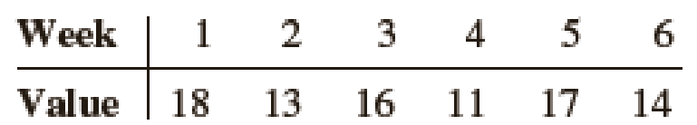
- a. Construct a time series plot. What type of pattern exists in the data?
- b. Develop the three-week moving average forecasts for this time series. Compute MSE and a forecast for week 7.
- c. Use α = .2 to compute the exponential smoothing forecasts for the time series. Compute MSE and a forecast for week 7.
- d. Compare the three-week moving average approach with the exponential smoothing approach using α = .2. Which appears to provide more accurate forecasts based on MSE? Explain.
- e. Use a smoothing constant of α = .4 to compute the exponential smoothing forecasts. Does a smoothing constant of .2 or .4 appear to provide more accurate forecasts based on MSE? Explain.
Expert Solution & Answer
Want to see the full answer?
Check out a sample textbook solution
Students have asked these similar questions
Consider the following time series data.
Week
1
2
3
4
5
6
Value
18
13
16
11
17
14
Construct a time series plot. What type of pattern exist in the data?
Develop a three-week moving average for this time series. Compute MSE and forecast for week 7.
Use a = 0.2 to compute the exponential smoothing values for the time series. Compute MSE and forecast for week 7.
Which of the following time series forecasting methods would not be used to forecast seasonal data?
consider the following time series data.Month 1 2 3 4 5 6 7Value 24 13 20 12 19 23 15a. compute MSe using the most recent value as the forecast for the next period. Whatis the forecast for month 8?b. compute MSe using the average of all the data available as the forecast for the nextperiod. What is the forecast for month 8?c. Which method appears to provide the better forecast?
Chapter 17 Solutions
Modern Business Statistics with Microsoft Office Excel (with XLSTAT Education Edition Printed Access Card) (MindTap Course List)
Ch. 17.2 - 1. Consider the following time series...Ch. 17.2 - 2. Refer to the time series data in exercise 1....Ch. 17.2 - Prob. 3ECh. 17.2 - 4. Consider the following time series...Ch. 17.3 - Consider the following time series...Ch. 17.3 - Consider the following time series...Ch. 17.3 - Refer to the gasoline sales time series data in...Ch. 17.3 - Prob. 8ECh. 17.3 - 9. With the gasoline time series data from Table...Ch. 17.3 - 10. With a smoothing constant of α = .2, equation...
Ch. 17.3 - For the Hawkins Company, the monthly percentages...Ch. 17.3 - Corporate triple-A bond interest rates for 12...Ch. 17.3 - The values of Alabama building contracts (in $...Ch. 17.3 - The following time series shows the sales of a...Ch. 17.3 - Ten weeks of data on the Commodity Futures Index...Ch. 17.3 - Prob. 16ECh. 17.4 - Consider the following time series...Ch. 17.4 - Prob. 18ECh. 17.4 - Prob. 19ECh. 17.4 - Prob. 20ECh. 17.4 - Prob. 21ECh. 17.4 - Prob. 22ECh. 17.4 - The president of a small manufacturing firm is...Ch. 17.4 - The following data shows the average interest rate...Ch. 17.4 - Quarterly revenue ($ millions) for Twitter for the...Ch. 17.4 - Giovanni Food Products produces and sells frozen...Ch. 17.4 - The number of users of Facebook from 2004 through...Ch. 17.5 - Consider the following time series.
Construct a...Ch. 17.5 - Consider the following time series...Ch. 17.5 - The quarterly sales data (number of copies sold)...Ch. 17.5 - Air pollution control specialists in southern...Ch. 17.5 - South Shore Construction builds permanent docks...Ch. 17.5 - Prob. 33ECh. 17.5 - Prob. 34ECh. 17.6 - Consider the following time series...Ch. 17.6 - Refer to exercise 35.
Deseasonalize the time...Ch. 17.6 - The quarterly sales data (number of copies sold)...Ch. 17.6 - Three years of monthly lawn-maintenance expenses...Ch. 17.6 - Air pollution control specialists in southern...Ch. 17.6 - Electric power consumption is measured in...Ch. 17 - The weekly demand (in cases) for a particular...Ch. 17 - The following table reports the percentage of...Ch. 17 - United Dairies, Inc., supplies milk to several...Ch. 17 - Annual retail store revenue for Apple from 2007 to...Ch. 17 - The Mayfair Department Store in Davenport, Iowa,...Ch. 17 - Prob. 47SECh. 17 - The Costello Music Company has been in business...Ch. 17 - Consider the Costello Music Company problem in...Ch. 17 - Prob. 50SECh. 17 - Refer to the Costello Music Company time series in...Ch. 17 - Prob. 52SECh. 17 - Refer to the Hudson Marine problem in exercise 52....Ch. 17 - Refer to the Hudson Marine problem in exercise...Ch. 17 - Refer to the Hudson Marine data in exercise...Ch. 17 - Forecasting Food and Beverage Sales
The Vintage...Ch. 17 - The Carlson Department Store suffered heavy damage...
Knowledge Booster


Learn more about
Need a deep-dive on the concept behind this application? Look no further. Learn more about this topic, statistics and related others by exploring similar questions and additional content below.Similar questions
- Consider the following time series data Week 1 2 3 4 5 6 Value 18 13 16 11 17 14 a. Construct a time series plot. What type of pattern exists in the data?b. Develop the three-week moving average forecasts for this time series. compute MSE and a forecast for week 7.c. Use α = .2 to compute the exponential smoothing forecasts for the time series.Compute MSE and a forecast for week 7.d. Compare the three-week moving average approach with the exponentialsmoothing approach using α = .2. Which appears to provide more accurate forecasts based on MSE? explain.e. Use a smoothing constant of α = .4 to compute the exponential smoothing forecasts. does a smoothing constant of .2 or .4 appear to provide more accurate forecasts based on MSE? explain.arrow_forwardConsider the following time series data: 1 2 3 4 5 6 7 26 15 22 14 21 25 17 PART 1.Compute MSE using the most recent value as the forecast for the next period and then calculate the forecast for month 8. PART 2.Compute MSE using the average of all the data available as the forecast for the next period. What is the forecast for month 8?arrow_forwardConsider the following time series data. Week 1 2 3 4 5 6 Value 18 13 16 11 17 14 a. Construct a time series plot. What type of pattern exists in thedata?b. Develop the three-week moving average forecasts for this timeseries. compute MSE and a forecast for week 7.c. Use α= .2 to compute the exponential smoothing forecasts for the time series. Compute MSE and a forecast for week 7.d. Compare the three-week moving average approach with theexponential smoothing approach using α = .2. Which appears to provide more accurate forecasts based on MSE? explain.e. Use a smoothing constant of α = .4 to compute the exponentialsmoothing forecasts. does a smoothing constant of .2 or .4 appearto provide more accurate forecasts based on MSE? explain.arrow_forward
- consider the following time series data.Month 1 2 3 4 5 6 7Value 24 13 20 12 19 23 15construct a time series plot. What type of pattern exists in the data?a. develop the three-week moving average forecasts for this time series. compute MSeand a forecast for week 8.b. Use a = .2 to compute the exponential smoothing forecasts for the time series. compute MSe and a forecast for week 8.c. compare the three-week moving average approach with the exponential smoothing approach using a = .2. Which appears to provide more accurate forecasts based on MSe?d. Use a smoothing constant of a = .4 to compute the exponential smoothing forecasts.does a smoothing constant of .2 or .4 appear to provide more accurate forecasts basedon MSe? explainarrow_forwardThe following data set provides the total number of shipments of core major household appliances in the U.S. from 2000 to 2016 (in millions): Year Shipments (millions) 2000 38.4 2001 38.2 2002 40.8 2003 42.5 2004 46.1 2005 47.0 2006 46.7 2007 44.1 2008 39.8 2009 36.5 2010 38.2 2011 36.0 2012 35.8 2013 39.2 2014 41.5 2015 42.9 2016 44.7 a. Plot the time series. b. Fit a three-year moving average to the data and plot the results. c. Fit a five-year moving average to the data and plot the results. d. Compute a linear trend forecasting equation and plot the trend line. e. Compute a quadratic trend forecasting equation and plot the results.arrow_forwardAfter its move in 1990 to La Junta, Colorado, and its new initiatives, the DeBourgh Manufacturing Company began an upward climb of record sales. Suppose the figures shown here are the DeBourgh monthly sales figures from January 2001 through December 2009 (in $1,000s). a) Produce a time series plot. Are there any trends evident in the data? Does DeBourgh have a seasonal component to its sales? b) Deseasonalize the data using Multiplicative model with a 0.5 weighted moving average. Produce a time series plot of the deseasonalized data and add a trendline. c) Forecast the sales from January to December of the year 2010. d) Include a discussion of the general direction of sales and any seasonal tendencies that might be occurrinG Month 2001 2002 2003 2004 2005 2006 2007 2008 2009 January 139.7 165.1 177.8 228.6 266.7 431.8 381 431.8 495.3 February 114.3 177.8 203.2 254 317.5 457.2 406.4 444.5 533.4 March 101.6 177.8 228.6 266.7 368.3 457.2 431.8 495.3 635 April 152.4 203.2…arrow_forward
- Which of the time series forecasting methods would not be used to forecast seasonal data?arrow_forwardConsider the following time series data. (07)Month 1 2 3 4 5 6 7 8 9value 23 12 20 22 15 23 24 17 22 a. Develop the three-week moving average forecasts for this time series. Compute MSE and a forecast for week 10.b. Use α = .2 to compute the exponential smoothing forecasts for the time series. Compute MSE and a forecast for week 10.c. Compare the three-week moving average approach with the exponential smoothing approach using α = .2. Which appears to provide more accurate forecasts based on MSE?arrow_forwardBelow you are given the first five values of a quarterly time series. The multiplicative model is appropriate and a four-quarter moving average will be used. Year Quarter Time Series Value Yt 1 1 36 2 24 3 16 2 4 20 1 44 An estimate of the combined trend-cycle component (T2Ct) for Quarter 3 of Year 1 (used for estimating the de-trended values), when a four-quarter moving average is used, is a. 24. b. 26. c. 28. d. 25.arrow_forward
- Consider the following time series data: Month 1 2 3 4 5 6 7 Value 23 14 19 12 20 24 15 (a) Compute MSE using the most recent value as the forecast for the next period. If required, round your answer to one decimal place. What is the forecast for month 8? If required, round your answer to one decimal place. Do not round intermediate calculation. (b) Compute MSE using the average of all the data available as the forecast for the next period. If required, round your answer to one decimal place. Do not round intermediate calculation. What is the forecast for month 8? If required, round your answer to one decimal place. (c) Which method appears to provide the better forecast? - Select your answer -NaïveAll data averageItem 5arrow_forwardConsider the following time series data: Month 1 2 3 4 5 6 7 Value 23 14 19 12 20 24 15 (a) Compute MSE using the most recent value as the forecast for the next period. If required, round your answer to one decimal place. What is the forecast for month 8? If required, round your answer to one decimal place. Do not round intermediate calculation. (b) Compute MSE using the average of all the data available as the forecast for the next period. If required, round your answer to one decimal place. Do not round intermediate calculation. What is the forecast for month 8? If required, round your answer to one decimal place.arrow_forwardconsider the following time series data.t 1 2 3 4 5 6 7yt10 9 7 8 6 4 4a. construct a time series plot. What type of pattern exists in the data?b. develop the linear trend equation for this time series.c. What is the forecast for t = 8?arrow_forward
arrow_back_ios
SEE MORE QUESTIONS
arrow_forward_ios
Recommended textbooks for you
 MATLAB: An Introduction with ApplicationsStatisticsISBN:9781119256830Author:Amos GilatPublisher:John Wiley & Sons Inc
 Probability and Statistics for Engineering and th...StatisticsISBN:9781305251809Author:Jay L. DevorePublisher:Cengage Learning
 Statistics for The Behavioral Sciences (MindTap C...StatisticsISBN:9781305504912Author:Frederick J Gravetter, Larry B. WallnauPublisher:Cengage Learning
 Elementary Statistics: Picturing the World (7th E...StatisticsISBN:9780134683416Author:Ron Larson, Betsy FarberPublisher:PEARSON
 The Basic Practice of StatisticsStatisticsISBN:9781319042578Author:David S. Moore, William I. Notz, Michael A. FlignerPublisher:W. H. Freeman
 Introduction to the Practice of StatisticsStatisticsISBN:9781319013387Author:David S. Moore, George P. McCabe, Bruce A. CraigPublisher:W. H. Freeman
MATLAB: An Introduction with Applications
Statistics
ISBN:9781119256830
Author:Amos Gilat
Publisher:John Wiley & Sons Inc
Probability and Statistics for Engineering and th...
Statistics
ISBN:9781305251809
Author:Jay L. Devore
Publisher:Cengage Learning
Statistics for The Behavioral Sciences (MindTap C...
Statistics
ISBN:9781305504912
Author:Frederick J Gravetter, Larry B. Wallnau
Publisher:Cengage Learning
Elementary Statistics: Picturing the World (7th E...
Statistics
ISBN:9780134683416
Author:Ron Larson, Betsy Farber
Publisher:PEARSON
The Basic Practice of Statistics
Statistics
ISBN:9781319042578
Author:David S. Moore, William I. Notz, Michael A. Fligner
Publisher:W. H. Freeman
Introduction to the Practice of Statistics
Statistics
ISBN:9781319013387
Author:David S. Moore, George P. McCabe, Bruce A. Craig
Publisher:W. H. Freeman
Time Series Analysis Theory & Uni-variate Forecasting Techniques; Author: Analytics University;https://www.youtube.com/watch?v=_X5q9FYLGxM;License: Standard YouTube License, CC-BY
Operations management 101: Time-series, forecasting introduction; Author: Brandoz Foltz;https://www.youtube.com/watch?v=EaqZP36ool8;License: Standard YouTube License, CC-BY