
Videos
An interesting and practical use of the χ2 test comes about in testing for segregation of species of plants or animals. Suppose that two species of plants, A and B, are growing on a test plot. To assess whether the species tend to segregate, a researcher randomly samples n plants from the plot; the species of each sampled plant, and the species of its nearest neighbor are recorded. The data are then arranged in a table, as shown here.
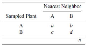
If a and d are large relative to b and c, we would be inclined to say that the species tend to segregate. (Most of A’s neighbors are of type A, and most of B’s neighbors are of type B.) If b and c are large compared to a and d, we would say that the species tend to be overly mixed. In either of these cases (segregation or overmixing), a χ2 test should yield a large value, and the hypothesis of random mixing would be rejected. For each of the following cases, test the hypothesis of random mixing (or, equivalently, the hypothesis that the species of a sample plant is independent of the species of its nearest neighbor). Use α = .05 in each case.
- a a = 20, b = 4, c = 8, d = 18.
- b a = 4, b = 20, c = 18, d = 8.
- c a = 20, b = 4, c = 18, d = 8.
Want to see the full answer?
Check out a sample textbook solution
Chapter 14 Solutions
Mathematical Statistics with Applications


- For the following table of data. x 1 2 3 4 5 6 7 8 9 10 y 0 0.5 1 2 2.5 3 3 4 4.5 5 a. draw a scatterplot. b. calculate the correlation coefficient. c. calculate the least squares line and graph it on the scatterplot. d. predict the y value when x is 11.arrow_forwardUrban Travel Times Population of cities and driving times are related, as shown in the accompanying table, which shows the 1960 population N, in thousands, for several cities, together with the average time T, in minutes, sent by residents driving to work. City Population N Driving time T Los Angeles 6489 16.8 Pittsburgh 1804 12.6 Washington 1808 14.3 Hutchinson 38 6.1 Nashville 347 10.8 Tallahassee 48 7.3 An analysis of these data, along with data from 17 other cities in the United States and Canada, led to a power model of average driving time as a function of population. a Construct a power model of driving time in minutes as a function of population measured in thousands b Is average driving time in Pittsburgh more or less than would be expected from its population? c If you wish to move to a smaller city to reduce your average driving time to work by 25, how much smaller should the city be?arrow_forward
 Calculus For The Life SciencesCalculusISBN:9780321964038Author:GREENWELL, Raymond N., RITCHEY, Nathan P., Lial, Margaret L.Publisher:Pearson Addison Wesley,
 Functions and Change: A Modeling Approach to Coll...AlgebraISBN:9781337111348Author:Bruce Crauder, Benny Evans, Alan NoellPublisher:Cengage Learning
 Holt Mcdougal Larson Pre-algebra: Student Edition...AlgebraISBN:9780547587776Author:HOLT MCDOUGALPublisher:HOLT MCDOUGAL