Subpart (a):
Profit maximization.
Subpart (a):
Explanation of Solution
Table – 1 represents the value of quantity, total cost, and total revenue.
Table – 1
| Quantity | Total cost | Total revenue |
| 0 | 8 | 0 |
| 1 | 9 | 8 |
| 2 | 10 | 16 |
| 3 | 11 | 24 |
| 4 | 13 | 32 |
| 5 | 19 | 40 |
| 6 | 27 | 48 |
| 7 | 37 | 56 |
The profit can be calculated by using the following formula:
Substitute the respective value in equation (1) and calculate the profit.
The profit is –$8.
Table – 2 shows the value of the profit that is obtained, by using equation (1).
Table – 2
| Quantity | Total cost | Total revenue | Profit |
| 0 | 8 | 0 | –8 |
| 1 | 9 | 8 | –1 |
| 2 | 10 | 16 | 6 |
| 3 | 11 | 24 | 13 |
| 4 | 13 | 32 | 19 |
| 5 | 19 | 40 | 21 |
| 6 | 27 | 48 | 21 |
| 7 | 37 | 56 | 19 |
From the above table, the firm can maximize profit when they produce five or six units of output.
Concept introduction:
Perfect competitive firm:
Marginal Revenue (MR): Marginal revenue refers to the additional revenue earned due to increasing one more unit of output.
Marginal Cost (MC): The marginal cost refers to the amount of an additional cost incurred in the process of increasing one more unit of output.
Subpart (b):
Profit maximization.
Subpart (b):
Explanation of Solution
The marginal revenue can be calculated by using the following formula:
Substitute the respective value in equation (2) and calculate marginal revenue.
The marginal revenue is $8.
Table – 3 shows the value of the marginal revenue that obtained by using equation (2).
Table – 3
| Quantity | Total cost | Total revenue | Marginal revenue | Profit |
| 0 | 8 | 0 | – | –8 |
| 1 | 9 | 8 | 8 | –1 |
| 2 | 10 | 16 | 8 | 6 |
| 3 | 11 | 24 | 8 | 13 |
| 4 | 13 | 32 | 8 | 19 |
| 5 | 19 | 40 | 8 | 21 |
| 6 | 27 | 48 | 8 | 21 |
| 7 | 37 | 56 | 8 | 19 |
The marginal cost can be calculated by using the following formula:
Substitute the respective value in equation (3) and calculate the marginal cost.
The marginal cost is $8.
Table – 4 shows the value of the marginal cost that is obtained by using equation (3).
Table – 4
| Quantity | Total cost | Marginal cost | Total revenue | Marginal revenue | Profit |
| 0 | 8 | – | 0 | – | –8 |
| 1 | 9 | 1 | 8 | 8 | –1 |
| 2 | 10 | 1 | 16 | 8 | 6 |
| 3 | 11 | 1 | 24 | 8 | 13 |
| 4 | 13 | 2 | 32 | 8 | 19 |
| 5 | 19 | 6 | 40 | 8 | 21 |
| 6 | 27 | 8 | 48 | 8 | 21 |
| 7 | 37 | 10 | 56 | 8 | 19 |
Figure – 1 shows the marginal revenue curve and marginal cost curve.
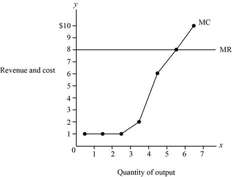
Figure – 1
From the above figure, the x axis shows the quantity of output and the y axis shows the price, that is, revenue and cost. From the above figure, the intersecting point shows the point the firm’s maximizing profit when they produce five or six units of output.
Concept introduction:
Perfect competitive firm: Perfect competition refers to the market structure featuring more number of sellers and buyers in the market, where the firm can sell homogenous products.
Marginal Revenue (MR): Marginal revenue refers to the additional revenue earned due to increasing one more unit of output.
Marginal Cost (MC): The marginal cost refers to the amount of an additional cost incurred in the process of increasing one more unit of output.
Subpart (c):
Profit in the long run.
Subpart (c):
Explanation of Solution
Since the marginal revenue is the same as each level of the quantity, the firm is in a competitive industry. The firm is earning an economic profit. Generally, firms in the long run earn a normal profit. Thus, the firm is not in the long run equilibrium.
Concept introduction:
Long run: Thelong run refers to the time, which changes the production variable to adjust to the market situation.
Want to see more full solutions like this?
Chapter 14 Solutions
EBK STUDY GUIDE FOR MANKIW'S PRINCIPLES

- "The Hickory Cabinet and Furniture Company makes chairs. The fixed cost per month of making chairs is $7,500, and the variable cost per chair is $40. Price is related to demand, according to the following linear equation: v = 400 - 1.2p Graphically illustrate the profit curve developed . Indicate the optimal price and the maximum profit per month.arrow_forwardFill in the blank boxes in the below chart given the information provided in the chart. You need to state and define ALL the cost relationships between Marginal Cost, Total Cost (TC), Total Variable Cost (TVC), and Total Fixed Cost (TFC); and Average Total Cost (ATC), Average Variable Cost (AVC), and Average Fixed Cost (AFC). For Average costs you should also use price and quantity relationships to define AFC, AVC and ATC.arrow_forwardQuestion 4 Use the following table for the (i),(ii) and (iii) questions. Quantity Total fixed cost Total variable cost 0 $800 $0 1 $800 $50 2 $800 $100 3 $800 $150 4 $800 $200 (i) What is the marginal cost of the third unit? A: $0 B: $50 C: $150 D: $250 (ii) What is the average total cost at the quantity of 4? A: $100 B: $150 C: $200 D: $250 (iii) From the information in the table above, is the marginal product diminishing? A: Yes, because the total cost is increasing as the quantity increases. B: Yes, because the total variable cost is increasing as the quantity increases. C: No, because the marginal cost is not increasing as quantity increases. D: No, because the total fixed cost is not increasing as quantity increases.arrow_forward
- Graphically show the relationship between the total fixed cost, the total variable cost, and the total cost. Draw a total cost curve and total revenue curve so that at some outputs that the firm takes losses, outputs where the firm makes unnecessary profits, and where the firm makes only necessary profits. Then, pick a point where the firm is taking losses and show on the graph, the firm’s total losses. Do the same for a point (an output level) where the firm may be making unnecessary profits.arrow_forwardWhat is relationship between total revenue (TR) and total variable cost (VC) if the price is less than AVC (is TR greater, less, or equal to VC)?arrow_forwardTotal Cost Marginal Cost (Dollars) Average Variable Cost (Dollars per pair) Fixed Cost Variable Cost Average Total Cost (Dollars per pair) Quantity (Pairs) (Dollars) (Dollars) (Dollars) 120 80 1 200 40 2 240 45 3 285 55 4 340 85 425 115 6 540 On the following graph, plot Douglas Fur's average total cost (ATC) curve using the green points (triangle symbol). Next, plot its average variable cost (AVC) curve using the purple points (diamond symbol). Finally, plot its marginal cost (MC) curve using the orange points (square symbol). (Hint: For ATC and AVC, plot the points on the integer; for example, the ATC of producing one pair of boots is $200, so you should start your ATC curve by placing a green point at (1, 200). For MC, plot the points between the integers: For example, the MC of increasing production from zero to one pair of boots is $80, so you should start your MC curve by placing an orange square at (0.5, 80).) Note: Plot your points in the order in which you would like them…arrow_forward
- Suppose the imaginary company of Athena is a small, Rochester-based American apparel manufacturer specializing in athleisure. The following table presents the brand's total cost of production at several different quantities. Fill in the remaining cells of the following table. Quantity Total Cost Marginal Cost Fixed Cost Variable Cost (Pairs) (Dollars) (Dollars) (Dollars) (Dollars) COSTS (Dollars per pair) 240 On the following graph, plot Douglas Fur's average total cost (ATC) curve using the green points (triangle symbol). Next, plot its average variable cost (AVC) curve using the purple points (diamond symbol). Finally, plot its marginal cost (MC) curve using the orange points (square symbol). (Hint: For ATC and AVC, plot the points on the integer; for example, the ATC of producing one pair of boots is $210, so you should start your ATC curve by placing a green point at (1, 210). For MC, plot the points between the integers: For example, the MC of increasing production from zero to…arrow_forwardQuestion 4 Pizza Inn Company Ltd is a new company in Accra that produces pizza, Lasagna, and Spaghetti Bolognese. The table below shows the production costs for the company. Use the table to answer the questions below Table 1: Cost for Producing Pizza Quantity Total Fixed Total Cost (TFC) Variable Cost (TVC) 1 2 3 4 5 6 60 60 60 60 60 60 Total Cost (TC) (AFC) Average Average Average Marginal Fixed Cost Variable Cost Cost (AC) (MC) 90 100 105 115 135 180 Cost (AVC) a) Fill in the cost table for Pizza Inn Company Ltd b) If the Pizza Inn operates under Perfect Competition and the market price is 20 (i.e. P=Gh20) what is the profit maximizing output level from the table c) Is this firm in the short run or long run and why? d) At the profit maximizing output level (found in A), is the firm making profit or loss; and what is the value of this profit or loss e) From your answer for D, should the firm shut down or continue to operate and why? (5 marks) f) Why is it that the Average Variable…arrow_forward1. Suppose marginal cost and average cost are given by the following expressions: MC(x)=3x1/2, AC(x)=2x1/2. What is the profit maximising quantity when p=$3?2. Suppose marginal cost and average cost are given by the following expressions: MC(x)=3x1/2, AC(x)=2x1/2. What is the value pf the long-run break-even price?3. For any given level of the price of output, the supply curve of a producer tells the producer the amount of output to produce in order to maximise profits a. True b. Falsearrow_forward
- Note: You need to show all your calculations within the table. Q1. Pizzas sell for $13 each. Pat's cost of producing pizzas is given below. Complete the table: Total Fixed Variable Average Marginal Total Marginal Output (pizzas per hour) Average Fixed Average Variable Cost Cost Cost Cost Cost Revenue Revenue (dollars per hour) (1) (2) (3) Cost Cost (6) (7) (8) (4) (5) 10 1 21 2 30 3 41 4 54 69 Write down the formulas for all the calculations in the table above, from columns 1-8:arrow_forward3. XYZ corporation produces widgets. Its short-run marginal cost curve is given by MC (q) = 10 – 5q + q² (this is a parabola whose minimum occurs at q = 2.5). XYZ's fixed costs are 10. In a two panel diagrams, graph the following cost curves: (a) total cost, (b) total variable cost, (c) total fixed cost, (d) marginal cost, (e) average variable cost, and (f) average total cost. Your diagrams do not need to be scale, but must be internally consistent (i.e. the relationships between different curves must be correct). You do not need to find mathematical expressions for the other cost curves – you only need to sketch lines that are consistent with the shape of the marginal cost curve.arrow_forwardWhat is relationship between total revenue (TR) and total variable cost (VC) if the price is equal to the AVC (tangent to the minimum AVC), (is TR greater, less, or equal to VC)? What do we call this point?arrow_forward
 Essentials of Economics (MindTap Course List)EconomicsISBN:9781337091992Author:N. Gregory MankiwPublisher:Cengage Learning
 Microeconomics: Principles & PolicyEconomicsISBN:9781337794992Author:William J. Baumol, Alan S. Blinder, John L. SolowPublisher:Cengage Learning