
Videos
a.
Check whether there is a positive linear relationship between the minimum and maximum width of an object.
a.
Answer to Problem 40E
There is convincing evidence that there is a positive linear relationship between the minimum and maximum width of an object.
Explanation of Solution
Calculation:
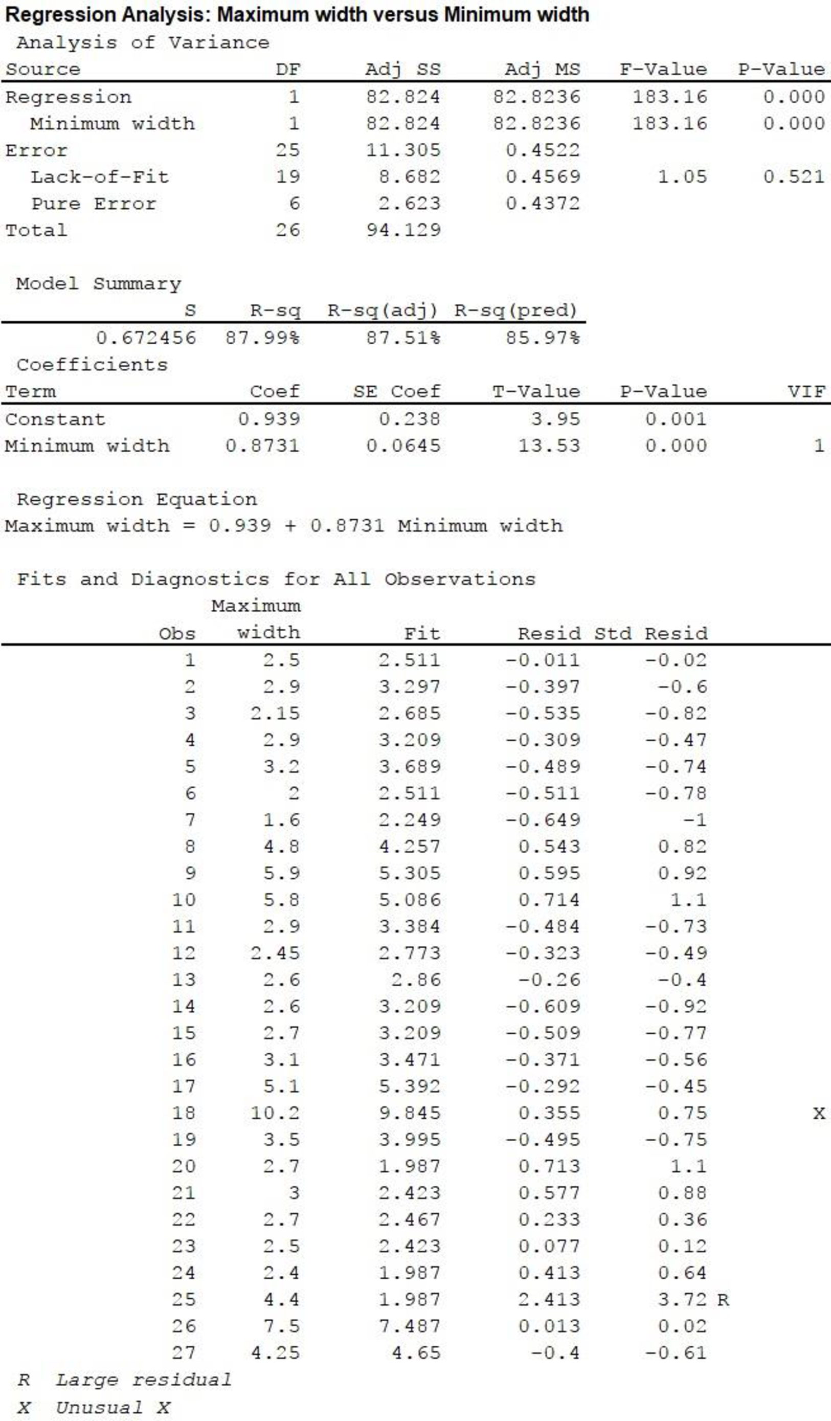
The given data provide the dimensions of 27 representative food products.
Here,
Null hypothesis:
That is, there is no linear relationship between the minimum and maximum width of an object.
Alternative hypothesis:
That is, there is a positive linear relationship between the minimum and maximum width of an object.
Here, the significance level is
Test Statistic:
The formula for test statistic is as follows:
In the formula, b denotes the estimated slope,
A standardized residual plot is shown below:
Standardized residual values and standardized residual plot:
Software procedure:
Step-by-step procedure to compute standardized residuals and its plot using MINITAB software:
- Select Stat > Regression > Regression > Fit Regression Model.
- In Response, enter the column of Maximum width.
- In Continuous Predictors, enter the columns of Minimum width.
- In Graphs, select Standardized under Residuals for Plots.
- In Results, select for all observations under Fits and diagnostics.
- In Residuals versus the variables, select Minimum width.
- Click OK.
Output obtained MINTAB software is given below:
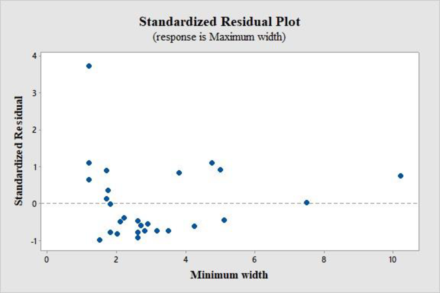
From the standardized residual plot, it is observed that one point lies outside the horizontal band of 3 units from the central line of 0. The standardized residual for this outlier is 3.72, that is, for product 25.
Assumption:
Here, the assumption made is that, the simple linear regression model is appropriate for the data, even though there is one extreme standardized residual.
Test Statistic:
In the MINITAB output, the test statistic value is displayed in the column “T-value” corresponding to “Minimum width”, in the section “Coefficients”. The value is 13.53.
P-value:
From the above output, the corresponding P-value is 0.
Rejection rule:
If
Conclusion:
The P-value is 0 and the level of significance is 0.05.
The P-value is less than the level of significance.
That is,
Therefore, reject the null hypothesis.
Thus, there is convincing evidence that there is a positive linear relationship between the minimum and maximum width of an object.
b.
Compute and interpret
b.
Answer to Problem 40E
Explanation of Solution
Calculation:
From the MINITAB output in Part (a), it is clear that
On an average, there is 67.246% deviation of the maximum width in the sample from the value predicted by least-squares regression.
c.
Find the 95% confidence interval for the mean maximum width of products for the minimum width of 6 cm.
c.
Answer to Problem 40E
The 95% confidence interval for the mean maximum width of products for the minimum width of 6 cm is (5.708, 6.647).
Explanation of Solution
Calculation:
The confidence interval for
From the MINITAB output in Part (a), the estimated linear regression line is
Point estimate:
The point estimate is calculated as follows:
Estimated standard deviation:
For the given x values, the summation values are given in the following table:
| Minimum width (X) | |
| 1.8 | 3.24 |
| 2.7 | 7.29 |
| 2 | 4 |
| 2.6 | 6.76 |
| 3.15 | 9.9225 |
| 1.8 | 3.24 |
| 1.5 | 2.25 |
| 3.8 | 14.44 |
| 5 | 25 |
| 4.75 | 22.5625 |
| 2.8 | 7.84 |
| 2.1 | 4.41 |
| 2.2 | 4.84 |
| 2.6 | 6.76 |
| 2.6 | 6.76 |
| 2.9 | 8.41 |
| 5.1 | 26.01 |
| 10.2 | 104.04 |
| 3.5 | 12.25 |
| 1.2 | 1.44 |
| 1.7 | 2.89 |
| 1.75 | 3.0625 |
| 1.7 | 2.89 |
| 1.2 | 1.44 |
| 1.2 | 1.44 |
| 7.5 | 56.25 |
| 4.25 | 18.0625 |
The value of
Substitute
Formula for degrees of freedom:
The formula for degrees of freedom is as follows:
The number of data value given is 27, that is
Critical value:
From the Appendix: Table of the t-critical values:
- Locate the value 25 in the degrees of freedom (df) column.
- Locate the 0.95 in the row of central area captured.
- The intersecting value that corresponds to df 25 with the confidence level 0.95 is 2.060.
Thus, the critical value for
Substitute
Therefore, one can be 95% confident that the mean maximum width of products with the minimum width of 6 cm will be between 5.708 cm and 6.647 cm.
d.
Find the 95% prediction interval for the mean maximum width of products with the minimum width of 6 cm.
d.
Answer to Problem 40E
The 95% prediction interval for the mean maximum width of products with the minimum width of 6 cm is (4.716, 7.640).
Explanation of Solution
Calculation:
The confidence interval for
The estimated standard deviation of the amount by which a single y observation deviates from the value predicted by an estimated regression line is
Substitute
From Part (c), the critical value for
Substitute
Therefore, the 95% prediction interval for the mean maximum width of products with the minimum width of 6 cm is (4.716, 7.640).
Want to see more full solutions like this?
Chapter 13 Solutions
Introduction to Statistics and Data Analysis


- A)Test the claim, at the a = 0.10 level of significance, that a linear relation exists between the two variables, for the data below, given that y-1.885x + 0.758. Step 1) State the null and alternative hypotheses. Step 2) Determine the critical value for the level of significance, a. Step 3) Find the test statistic or P-value. Step 4) Will the researcher reject the null hypothesis or do not the null hypothesis? Step 5) Write the conclusion. B) The regression line for the given data is y = -1.885x + 0.758. Determine the residual of a data point for which x = 2 and y = -4. C) Give a practical interpretation of the coefficient of determination, R2. Express R2 to the nearest whole percent. HIML Editor SAMSUNG &arrow_forwardA)Test the claim, at the a = 0.10 level of significance, that a linear relation exists between the two variables, for the data below, given that y-1.885x +0.758. -5 |-3| 4 11 6 y Step 1) State the null and alternative hypotheses. Step 2) Determine the critical value for the level of significance, a. Step 3) Find the test statistic or P-value. Step 4) Will the researcher reject the null hypothesis or do not the null hypothesis? Step 5) Write the conclusion. B) The regression line for the given data is v = -1.885x + 0.758. Determine the residual of a data point for which x = 2 and y = -4. SAMSUNG DII 96 &arrow_forward
 Linear Algebra: A Modern IntroductionAlgebraISBN:9781285463247Author:David PoolePublisher:Cengage Learning
 Calculus For The Life SciencesCalculusISBN:9780321964038Author:GREENWELL, Raymond N., RITCHEY, Nathan P., Lial, Margaret L.Publisher:Pearson Addison Wesley,
 Glencoe Algebra 1, Student Edition, 9780079039897...AlgebraISBN:9780079039897Author:CarterPublisher:McGraw Hill
 Big Ideas Math A Bridge To Success Algebra 1: Stu...AlgebraISBN:9781680331141Author:HOUGHTON MIFFLIN HARCOURTPublisher:Houghton Mifflin Harcourt