Find the degrees of freedom.
Obtain the critical value.
State the conclusion.
Answer to Problem 31CE
The degrees of freedom are 68.
The critical value is
The predictor ‘BachDeg%’ is significant.
Explanation of Solution
Calculation:
The given information is that, the dataset of ‘Noodles & Company Sales, Seating, and Demographic data’ contains
The formula for the test statistic for coefficient of predictor
Where,
The formula for degrees of freedom is,
Where, n is the total number of observations, k is the number of predictors.
Software procedure:
Step by step procedure to obtain test statistics using MegaStat software is given as,
- • Choose MegaStat >Correlation/Regression>Regression Analysis.
- • SelectInput ranges, enter the variable range for ‘Seats-Inside, Seats-Patio, MedIncome, MedAge, BachDeg%’ as the column of X, Independent variable(s)
- • Enter the variable range for ‘Sales/SqFt’ as the column of Y, Dependent variable.
- • Click OK.
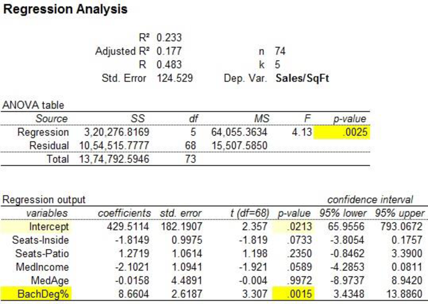
Output using MegaStatsoftware is given below:

The test statistic for predictor seats-inside is –1.819.
The test statistic for predictor seats-patio is 1.198.
The test statistic for predictor MedIncome is –1.921.
The test statistic for predictor MedAge is –0.004.
The test statistic for predictor BachDeg% is 3.307.
Substitute 74 for n, and 5 for k in the degrees of freedom formula.
The degrees of freedom are 68.
Software procedure:
Step by step procedure to obtain the critical value using MINITAB software is given as,
- • Choose Graph > Probability Distribution Plot choose View Probability > OK.
- • From Distribution, choose ‘t’ distribution.
- • In Degrees of freedom, enter 68.
- • Click the Shaded Area tab.
- • Choose probability and Two Tail for the region of the curve to shade.
- • Enter the data value as 0.05.
- • Click OK.
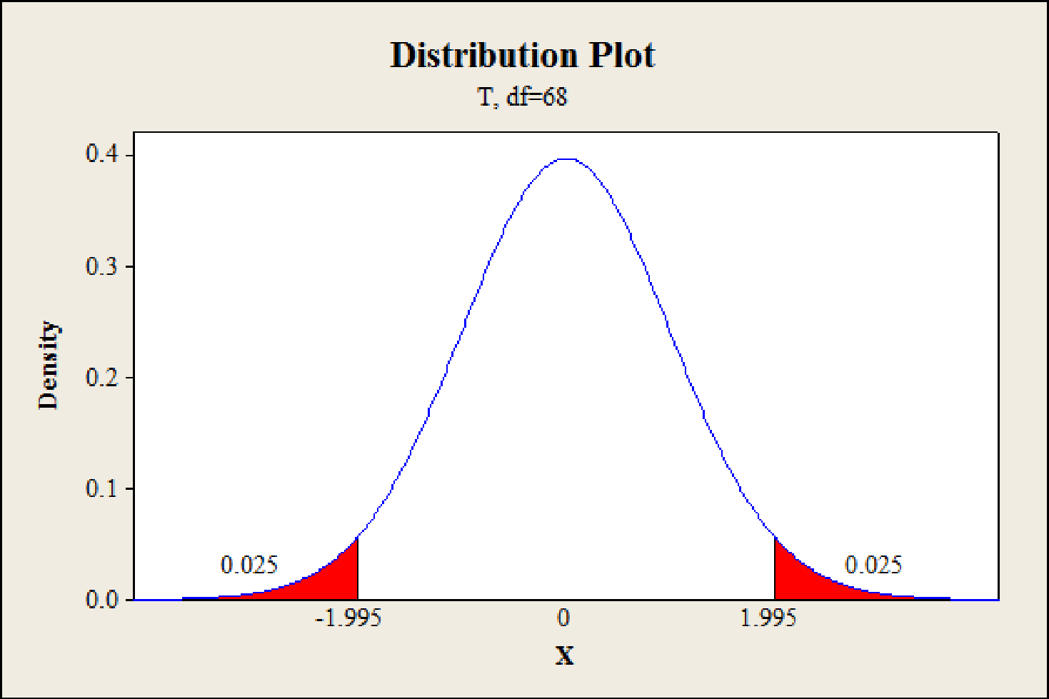
The output of the software is,

Hence, the critical value for 68 degrees of freedom with 0.05, level of significance is
Decision rules:
- • If test statistic value lies between positive and negative critical value, then do not reject null hypothesis.
- • Otherwise, reject the null hypothesis.
Coefficient of Seats-Inside:
That is variable Seats-Inside is not related to Sales/SqFt.
Alternative hypothesis:
That is variable Seats-Inside is related to Sales/SqFt.
Conclusion:
The value of test statistic is –1.819.
The critical values are –1.995 and 1.995.
The test statistic value lies between positive and negative critical value.
That is,
Hence the null hypothesis is not rejected.
The predictor Seats-Inside is not significant.
Coefficient of Seats-Patio:
That is variable Seats-Patio is not related to Sales/SqFt.
Alternative hypothesis:
That is variable Seats-Patio is related to Sales/SqFt.
Conclusion:
The value of test statistic is 1.198.
The critical values are –1.995 and 1.995.
The test statistic value lies between positive and negative critical value.
That is,
Hence the null hypothesis is not rejected.
The predictor Seats-Patio is not significant.
Coefficient of MedIncome:
That is variable MedIncome is not related to Sales/SqFt.
Alternative hypothesis:
That is variable MedIncome is related to Sales/SqFt.
Conclusion:
The value of test statistic is –1.921.
The critical values are –1.995 and 1.995.
The test statistic value lies between positive and negative critical value.
That is,
Hence the null hypothesis is not rejected.
The predictor MedIncome is not significant.
Coefficient of MedAge:
That is variable MedAge is not related to Sales/SqFt.
Alternative hypothesis:
That is variable MedAge is related to Sales/SqFt.
Conclusion:
The value of test statistic is –0.004.
The critical values are –1.995 and 1.995.
The test statistic value lies between positive and negative critical value.
That is,
Hence the null hypothesis is not rejected.
The predictor MedAge is not significant.
Coefficient of BachDeg%:
That is variable BachDeg% is not related to Sales/SqFt.
Alternative hypothesis:
That is variable BachDeg% is related to Sales/SqFt.
Conclusion:
The value of test statistic is 3.307.
The critical values are –1.995 and 1.995.
The test statistic value is greater than the positive critical value.
The test statistic value does not lie between positive and negative critical value.
That is,
Hence the null hypothesis is rejected.
The predictor BachDeg% is significant.
Hence, the predictor BachDeg% significantly from zero at
Want to see more full solutions like this?
Chapter 13 Solutions
Applied Statistics in Business and Economics
- AP1.2 A child is 40 inches tall, which places her at the 90th percentile of all children of similar age. The heights for children of this age form an approximately Normal distribution with a mean of 38 inches. Based on this information, what is the standard deviation of the heights of all children of this age? 0.20 inches (c) 0.65 inches (e) 1.56 inches 0.31 inches (d) 1.21 inchesarrow_forwardAP1.1 You look at real estate ads for houses in Sarasota, Florida. Many houses range from $200,000 to $400,000 in price. The few houses on the water, however, have prices up to $15 million. Which of the following statements best describes the distribution of home prices in Sarasota? The distribution is most likely skewed to the left, and the mean is greater than the median. The distribution is most likely skewed to the left, and the mean is less than the median. The distribution is roughly symmetric with a few high outliers, and the mean is approximately equal to the median. The distribution is most likely skewed to the right, and the mean is greater than the median. The distribution is most likely skewed to the right, and the mean is less than the median.arrow_forwardDuring busy political seasons, many opinion polls are conducted. In apresidential race, how do you think the participants in polls are generally selected?Discuss any issues regarding simple random, stratified, systematic, cluster, andconvenience sampling in these polls. What about other types of polls, besides political?arrow_forward
- Please could you explain why 0.5 was added to each upper limpit of the intervals.Thanksarrow_forward28. (a) Under what conditions do we say that two random variables X and Y are independent? (b) Demonstrate that if X and Y are independent, then it follows that E(XY) = E(X)E(Y); (e) Show by a counter example that the converse of (ii) is not necessarily true.arrow_forward1. Let X and Y be random variables and suppose that A = F. Prove that Z XI(A)+YI(A) is a random variable.arrow_forward
 Holt Mcdougal Larson Pre-algebra: Student Edition...AlgebraISBN:9780547587776Author:HOLT MCDOUGALPublisher:HOLT MCDOUGAL
 Glencoe Algebra 1, Student Edition, 9780079039897...AlgebraISBN:9780079039897Author:CarterPublisher:McGraw Hill
 Big Ideas Math A Bridge To Success Algebra 1: Stu...AlgebraISBN:9781680331141Author:HOUGHTON MIFFLIN HARCOURTPublisher:Houghton Mifflin Harcourt
 Functions and Change: A Modeling Approach to Coll...AlgebraISBN:9781337111348Author:Bruce Crauder, Benny Evans, Alan NoellPublisher:Cengage Learning


