To graph: The interaction plot displaying systolic blood pressure on the y -axis and training level on the x -axis.

Question

Want to see more full solutions like this?

Answer 1

Question

Definition Definition Measure of central tendency that is the average of a given data set. The mean value is evaluated as the quotient of the sum of all observations by the sample size. The mean, in contrast to a median, is affected by extreme values. Very large or very small values can distract the mean from the center of the data. Arithmetic mean: The most common type of mean is the arithmetic mean. It is evaluated using the formula: μ = 1 N ∑ i = 1 N x i Other types of means are the geometric mean, logarithmic mean, and harmonic mean. Geometric mean: The nth root of the product of n observations from a data set is defined as the geometric mean of the set: G = x 1 x 2 ... x n n Logarithmic mean: The difference of the natural logarithms of the two numbers, divided by the difference between the numbers is the logarithmic mean of the two numbers. The logarithmic mean is used particularly in heat transfer and mass transfer. ln x 2 − ln x 1 x 2 − x 1 Harmonic mean: The inverse of the arithmetic mean of the inverses of all the numbers in a data set is the harmonic mean of the data. 1 1 x 1 + 1 x 2 + ...

Chapter 13, Problem 18E

(a)

To determine

To graph: The interaction plot displaying systolic blood pressure on the y-axis and training level on the x-axis.

(a)

Expert Solution

Explanation of Solution

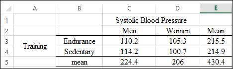
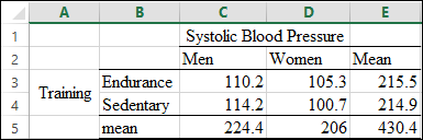
Graph: The problem compares two factors systolic blood pressure on y-axis with training level on x-axis. The factor systolic blood pressure is further classified for men and women and the other factor training level is classified to endurance trained and sedentary men and women. Thus, the table is created for the means of two factor as shown below;

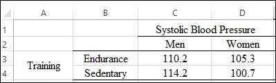
Introduction To The Practice Of Statistics, Chapter 13, Problem 18E , additional homework tip 1

The marginal means for Endurance is calculated by using the function $=SUM(C3:D3)$

Introduction To The Practice Of Statistics, Chapter 13, Problem 18E , additional homework tip 2

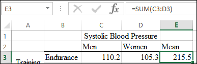
The marginal means for Sedentary is calculated by using the function $=SUM(C3:D3)$

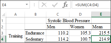
Introduction To The Practice Of Statistics, Chapter 13, Problem 18E , additional homework tip 3

The marginal means for Systolic blood pressure for men is calculated by using the function $=SUM(C3:D3)$

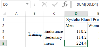
Introduction To The Practice Of Statistics, Chapter 13, Problem 18E , additional homework tip 4

The marginal means for Systolic blood pressure for women is calculated by using the function $=SUM(C3:D3)$

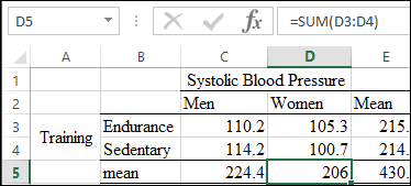
Introduction To The Practice Of Statistics, Chapter 13, Problem 18E , additional homework tip 5

The table is obtained as:

Introduction To The Practice Of Statistics, Chapter 13, Problem 18E , additional homework tip 6

The interaction plot is drawn by following these steps:

Step 1: Open Excel sheet and write the data value. The screenshot is shown below:

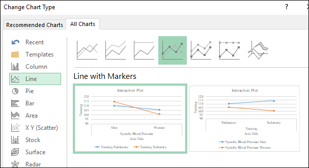
Introduction To The Practice Of Statistics, Chapter 13, Problem 18E , additional homework tip 7

Step 2: INSERT>Recommended Charts>All Charts>Line Chart. The screenshot is shown below:

Introduction To The Practice Of Statistics, Chapter 13, Problem 18E , additional homework tip 8

The interaction plot is obtained as shown below:

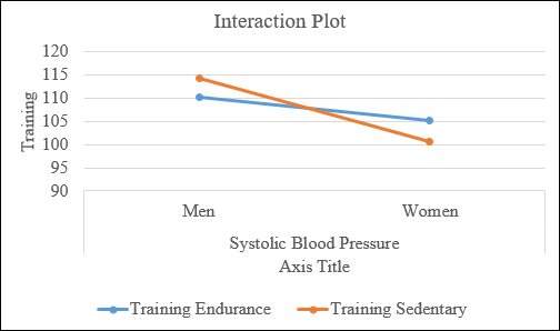
Introduction To The Practice Of Statistics, Chapter 13, Problem 18E , additional homework tip 9

Interpretation: From the chart above, the two lines are not parallel, hence, there is an interaction present between two factors. There is a main effect of training level, training sedentary takes much lower value for women when compared to training endurance for women.

(b)

To determine

To find: The ANOVA table.

(b)

Expert Solution

Answer to Problem 18E

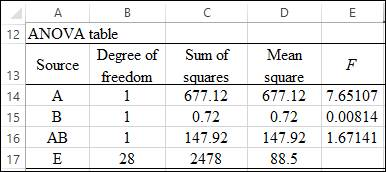
Solution: The ANOVA table is obtained as:

Introduction To The Practice Of Statistics, Chapter 13, Problem 18E , additional homework tip 10

Explanation of Solution

Given: The following values of the Sum of Squares is provided,

$SSA=677.12SSB=0.72SSAB=147.92SSE=2478$ ,

where A is the sex effect and B is the training level.

Calculation: The ANOVA table is obtained by following these steps:

Step 1: The degree of freedom for “A” is obtained as follows:

$DFA=I−1=2−1=1$

The degree of freedom for “B” is obtained as follows;

$DFB=J−1=2−1=1$

The degree of freedom for “AB” is obtained as follows:

$DFAB=(I−1)(J−1)=(2−1)×(2−1)=1$

The degree of freedom for “E” is obtained as follows:

$DFE=N−IJ=32−(2×2)=28$

Step 2: The mean squares for “A” is obtained as follows:

$MSA=SSADFA=677.121=677.12$

The mean squares for “B” is obtained as follows:

$MSB=SSBDFB=0.721=0.72$

The mean squares for “AB” is obtained as follows:

$MSAB=SSABDFAB=147.921=147.92$

The mean squares for “E” is obtained as follows:

$MSE=SSEDFE=247828=88.5$

Step 3: The F-value for “A” is obtained as follows:

$F=MSAMSE=677.1288.5=7.6511$

The F-value for “B” is obtained as follows:

$F=MSBMSE=0.7288.5=0.0081$

The F-value for “AB” is obtained as follows:

$F=MSABMSE=147.9288.5=1.6714$

To test the hypothesis for the obtained F-values, the F-critical value is obtained through the F-distribution table as $F(1,28)=4.19$

Interpretation: The comparisons of F-values with F-critical are as follows:

$FA>FcriticalFB<FcriticalFAB<Fcritical$

The value of F_A is greater than F-critical; hence, the null hypothesis can be rejected significantly, which states that there is a main effect of training level. While the other factor systolic blood pressure and the interaction of these two factors have F-value less than F-critical, which means that they do not show the significant difference in means.

(c)

To determine

The benefit of considering pretest measurement.

(c)

Expert Solution

Answer to Problem 18E

Solution: It increases the power of the test statistic.

Explanation of Solution

The benefit of pre/post measurement or repeated measure improves the test statistic by reducing the within group variability when comparing the mean differences. The power of the test statistic can be understood as the probability of detecting the significant difference when comparing means, increases as a result of reduction in variance of means.

Want to see more full solutions like this?

Subscribe now to access step-by-step solutions to millions of textbook problems written by subject matter experts!

Students have asked these similar questions

Can you help me solve problem 38 with steps im stuck.

How do the samples hold up to the efficiency test? What percentages of the samples pass or fail the test? What would be the likelihood of having the following specific number of efficiency test failures in the next 300 processors tested? 1 failures, 5 failures, 10 failures and 20 failures.

The battery temperatures are a major concern for us. Can you analyze and describe the sample data? What are the average and median temperatures? How much variability is there in the temperatures? Is there anything that stands out? Our engineers’ assumption is that the temperature data is normally distributed. If that is the case, what would be the likelihood that the Safety Zone temperature will exceed 5.15 degrees? What is the probability that the Safety Zone temperature will be less than 4.65 degrees? What is the actual percentage of samples that exceed 5.25 degrees or are less than 4.75 degrees? Is the manufacturing process producing units with stable Safety Zone temperatures? Can you check if there are any apparent changes in the temperature pattern? Are there any outliers? A closer look at the Z-scores should help you in this regard.

Answer 2