System Dynamics
System Dynamics
3rd Edition
ISBN: 9780073398068
Author: III William J. Palm
Publisher: MCG
bartleby

Concept explainers

Question
Book Icon
Chapter 13, Problem 13.23P
To determine

(a)

The expression for X1(jω)F(jω).

The expression for X2(jω)F(jω).

Expert Solution
Check Mark

Answer to Problem 13.23P

The expression for X1(jω)F(jω) is (λμr2)2+(2ςr)2|[μr4(1+λ+μλ)r2+μα2]2+[(2ςr)2(1(1+μ)r2)]2|.

The expression for X2(jω)F(jω) is |(λ2+(2ςrj)2)||[μr4(1+λ+μλ)r2+μα2]2+[(2ςr)2(1(1+μ)r2)]2|.

Explanation of Solution

Given information:

The main mass is m1.

Write the expression for force of mass 1.

f=m1x¨1+c(x˙1x˙2)+k12x1+k12x1+k2(x1x2)f=m1x¨1+cx˙1+k1x1+k2x2k2x2cx˙2           ...... (I)

Here, mass of body 1 is m1, damping coefficient is c, velocity of mass 1 is x˙1, velocity of mass 2 is x˙2, stiffness is k, displacement is x, acceleration of mass 1 is x¨1 and the coefficient of friction is f.

Write the expression for absorber mass.

m2x¨2+cx˙2cx˙1+k2(x2x1)m2x¨2=cx˙2+cx˙1k2x2+k2x1          . (II)

Here, mass of the absorber is m2. and the acceleration of absorber is x¨2.

Apply Laplace transform on Equation (I).

L(f)=L[m1x¨1+cx˙1+k1x1+k2x2k2x2cx˙2]F(s)=(m1s2+cs+k1+k2)X1(s)(cs+k2)X2(s)           (III)

Take Laplace transform of equation (II).

L[m2x¨2]=L[cx˙2+cx˙1k2x2+k2x1]m2s2X2(s)=csX2(s)+csX1(s)k2X2(s)+k2X1(s)=0(cs+k2)X1(s)+(m2s2+cs+k2)X2(s)=0           .. (IV)

Apply Cramer rule in Equation (III) and (IV).

(m1s2+cs+k1+k2(cs+k2)(cs+k2)m2s2+cs+k2)(X1(s)X2(s))=(F(s)0)           ...... .. (V)

Further solve Equation (V).

D(s)=[m1m2s4+cm2s3+k1m2s2+k2m2s2+m1cs3+(cs)2+ck1s+k2cs+m1k2s2+k2cs+k1k2+k2k2(c2s2+k22+2ck2s)]D(s)=m1m2s4+c(m1+m2)s3+(m2k1+m2k2+m1k2)s2+ck1s+k1k2           (VI)

Write the expression for parameter μ.

μ=m2m1           ...... ... (VII)

Write the expression for parameter ω12.

ω12=k1m1           ...... .. (VIII)

Write the expression for parameter ς.

ς=c2m1k          . (IX)

Write the expression for parameter r.

r=ωω1           .. (X)

Here, angular speed of main mass is ω1.

Write the expression for parameter ω22.

ω22=k2m2           ...... .. (XI)

Write the expression for parameter λ.

λ=k2k1          . (XII)

Write the expression for parameter α.

α=ω1ω2          . (XIII)

Substitute jω for s in Equation (VI).

D(jω)=[(jω)(m1m2(jω)3+c(m2+m1)(jω)2+(m2k1+m2k2+m1k2)(jω)+ck1+k1k2)]=|m1m2ω4c(m2+m1)ω3j+(m2k1+m2k2+m1k2)ω2+ck1jω+k1k2|           ...... (XIV)

Substitute m2m1 for μ, km1 for ω12, ς for c2m1k, r for ωω1, ω22 for k2m2, λ for k2k1 and ω1ω2 for α in Equation (XIV).

D(jω)=|m12ω14[μr4(1+γ+μγ)+μα2]+[2ςr2(1+μ)r3]j|           (XV)

Apply Cramer rule for Equation (VI) to obtain D1(s).

D1(s)=(F(s)(cs+k2)0m2s2+cs+k2)=F(s)(m2s2+cs+k2)+0×((cs+k2))=F(s)(m2s2+cs+k2)          . (XVI)

Apply Cramer rule for Equation (VI) to obtain D2(s).

D2(s)=(m2s2+cs+k2+k1F(s)(cs+k2)0)=0×(m2s2+cs+k2+k1)F(s)×((cs+k2))=F(s)(cs+k2)          . (XVII)

Write the expression for X1(s).

X1(s)=D1(s)D(s)           ...... .. (XVIII)

Substitute F(s)(m2s2+cs+k2) for D1(s) and m1m2s4+c(m1+m2)s3+(m2k1+m2k2+m1k2)s2+ck1s+k1k2 for D(s) in equation (XVIII).

X1(s)=F(s)(m2s2+cs+k2)m1m2s4+c(m1+m2)s3+(m2k1+m2k2+m1k2)s2+ck1s+k1k2          . (XIX)

Substitute jω for s in Equation (XIX).

X1(jω)F(jω)=(m2(jω)2+cjω+k2)[m1m2(jω)4+c(m1+m2)(jω)3+(m2k1+m2k2+m1k2)(jω)2+ck1jω+k1k2]           (XX)

Substitute m2m1 for μ, km1 for ω12, ς for c2m1k, r for ωω1, ω22 for k2m2, λ for k2k1 and ω1ω2 for α in Equation (XIX).

k1X1(jω)F(jω)=(k1)2(λμr2)2+(2ςr)2m12ω14|[μr4(1+λ+μλ)r2+μα2]+[2ςr2(1+μ)r3]j| .... (XXI)

Substitute m1ω12 for k in Equation (XXI).

k1X1(jω)F(jω)=k12(λμr2)2+(2ςr)2k12|[μr4(1+λ+μλ)r2+μα2]+[2ςr2(1+μ)r3]j|k1X1(jω)F(jω)=(λμr2)2+(2ςr)2|[μr4(1+λ+μλ)r2+μα2]2+[(2ςr)2(1(1+μ)r2)]2| ......... (XXII)

Write the expression for X2(s).

X2(s)=D2(s)D(s)           ....... (XXIII)

Substitute F(s)(cs+k2) for D2(s) and m1m2s4+c(m1+m2)s3+(m2k1+m2k2+m1k2)s2+ck1s+k1k2 for D(s) in Equation (XXIII).

X2(s)=F(s)(cs+k2)[m1m2s4+c(m1+m2)s3+(m2k1+m2k2+m1k2)s2+ck1s+k1k2]X2(s)F(s)=(cs+k2)[m1m2s4+c(m1+m2)s3+(m2k1+m2k2+m1k2)s2+ck1s+k1k2] ........ (XXIV)

Substitute jω for, m2m1 for μ, km1 for ω12, ς for c2m1k, r for ωω1, ω22 for k2m2, λ for k2k1 and ω1ω2 for α in Equation (XXIV).

k1X2(jω)F(jω)=k1k1|(λ+2ςrj)|[m1m2ω4c(m1+m2)jω3(m2k1+m2k2+m1k2)ω2+ck1jω+k1k2]           ...... (XXV)

Solve Equation (XV) and (XXV).

k1X2(jω)F(jω)=k1k1|(λ+2ςrj)|m12ω14|[μr4(1+λ+μλ)r2+μα2]+[2ςr2(1+μ)r3]j| ....... (XXVI)

Substitute m1ω12 for k1 in RHS of Equation (XXVI).

k1X2(jω)F(jω)=m1ω12m1ω12|(λ+2ςrj)|m12ω14|[μr4(1+λ+μλ)r2+μα2]+[2ςr2(1+μ)r3]j|=|(λ+2ςrj)||[μr4(1+λ+μλ)r2+μα2]+[2ςr2(1+μ)r3]j|=|(λ2+(2ςrj)2)||[μr4(1+λ+μλ)r2+μα2]2+[(2ςr)2(1(1+μ)r2)]2|.

Conclusion:

The expression for X1(jω)F(jω) is (λμr2)2+(2ςr)2|[μr4(1+λ+μλ)r2+μα2]2+[(2ςr)2(1(1+μ)r2)]2|.

The expression for X2(jω)F(jω) is |(λ2+(2ςrj)2)||[μr4(1+λ+μλ)r2+μα2]2+[(2ςr)2(1(1+μ)r2)]2|.

To determine

(b)

The plot between kX1F and ωkm1.

Expert Solution
Check Mark

Answer to Problem 13.23P

The plot between kX1F and ωkm1 is shown in Figure-(1).

Explanation of Solution

Given information:

The main mass is m1 and the absorber mass is m2.

To plot the graph, consider some constant values such as 10 for m1, 30 for m2, 104 for k and [0,2] for r.

Calculation:

Substitute 10 for m1 and 30 for m2 in equation (VII).

μ=3010=0.3333

Substitute 104 for k and 10 for m1 in Equation (VIII).

ω12=10410ω12=1000ω1=1000ω1=31.6

Substitute 2×10⁴ for k2 in Equation (XI).

ω22=2×10430ω22=666.666ω=25.8

Substitute 2×10⁴ for k2 and 104 in equation (XII).

λ=2×104104=2

Substitute 31.6 for ω1 and 25.8 for ω in equation (XIII).

α=31.625.8=1.2

Assume 0 for ω and 0.1 for ς.

Substitute 0 for ω and 31.6 for ω1 in Equation (X).

r=031.6=0

Substitute 0 for r, 2 for λ, 0.3333 for μ, 1.2 for α and 0.1 for ς in Equation (XXII).

k1X1(jω)F(jω)=(2(0.3333)(0)2)2+(2×0.1×0)2|[[μ×04(1+2+0.3333×2)×02+0.3333×(1.2)2]2+[(2×0.1×0)2((1(1+0.3333))02)]2]|=20.234.16

Substitute 10 for m, 0.3 for ς and 104 in Equation (IX).

0.3=2210×104c=210×104×0.3c=1789.7

Prepare a table for various value of k1X1F1, ωkm1 and ς.

ω ς kX1(jω)F(jω) ωkm1
0 0.1 4.2 0
10 0.1 0.61 0.316
20 0.1 1.99 0.633
30 0.1 0.67 0.949
0 0.3 4.16 0
10 0.3 0.61 0.316
20 0.3 2 0.633
30 0.3 0.7 0.949
0 0.5 4.16 0
10 0.5 0.62 0.316
20 0.5 2.01 0.633
30 0.5 0.76 0.949
0 1 4.16 0
10 1 0.64 0.316
20 1 2.04 0.633
30 1 0.98 0.949

The figure below shows the plot between
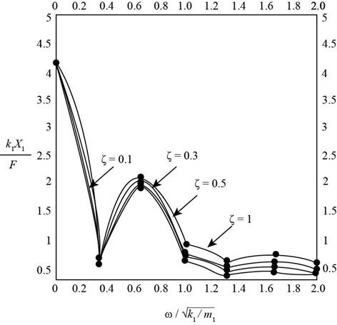
 k1X1F1 and ωkm1.

System Dynamics, Chapter 13, Problem 13.23P , additional homework tip  1

        Figure-(1)

Conclusion:

The plot between k1X1F1 and ωkm1 is shown below.

System Dynamics, Chapter 13, Problem 13.23P , additional homework tip  2

        Figure-(1).

Want to see more full solutions like this?

Subscribe now to access step-by-step solutions to millions of textbook problems written by subject matter experts!
Knowledge Booster
Background pattern image
Mechanical Engineering
Learn more about
Need a deep-dive on the concept behind this application? Look no further. Learn more about this topic, mechanical-engineering and related others by exploring similar questions and additional content below.
Recommended textbooks for you
Text book image
Elements Of Electromagnetics
Mechanical Engineering
ISBN:9780190698614
Author:Sadiku, Matthew N. O.
Publisher:Oxford University Press
Text book image
Mechanics of Materials (10th Edition)
Mechanical Engineering
ISBN:9780134319650
Author:Russell C. Hibbeler
Publisher:PEARSON
Text book image
Thermodynamics: An Engineering Approach
Mechanical Engineering
ISBN:9781259822674
Author:Yunus A. Cengel Dr., Michael A. Boles
Publisher:McGraw-Hill Education
Text book image
Control Systems Engineering
Mechanical Engineering
ISBN:9781118170519
Author:Norman S. Nise
Publisher:WILEY
Text book image
Mechanics of Materials (MindTap Course List)
Mechanical Engineering
ISBN:9781337093347
Author:Barry J. Goodno, James M. Gere
Publisher:Cengage Learning
Text book image
Engineering Mechanics: Statics
Mechanical Engineering
ISBN:9781118807330
Author:James L. Meriam, L. G. Kraige, J. N. Bolton
Publisher:WILEY