
Concept explainers
Videos
The paper “Sociochemosensory and Emotional
One of the three shirts had been worn by the subject’s roommate. The subject was asked to identify the shirt worn by her roommate. This process was then repeated with another three shirts, and the number of times out of the two trials that the subject correctly identified the shirt worn by her roommate was recorded. The resulting data are summarized in the accompanying table.
![Chapter 12.1, Problem 10E, The paper Sociochemosensory and Emotional Functions (Psychological Science [2009]: 11181124)](https://content.bartleby.com/tbms-images/9781337793612/Chapter-12/images/93612-12.1-10e-question-digital_image_001.png)
- a. Can a person identify her roommate by smell? If not, the data from the experiment should be consistent with what we would have expected to see if subjects were just guessing on each trial. That is, we would expect that the probability of selecting the correct shirt would be 1/3 on each of the two trials.
Calculate the proportions of the time we would expect to see 0, 1, and 2 correct identifications if subjects are just guessing. (Hint: 0 correct identifications occurs if the first trial is incorrect and the second trial is incorrect.)
- b. Use the three proportions calculated in Part (a) to carry out a test to determine if the numbers of correct identifications by the students in this study are significantly different from what would have been expected by guessing. Use α = 0.05. (Note: One of the expected counts is just a bit less than 5. For purposes of this exercise, assume that it is OK to proceed with a goodness-of-fit test.)
a.
Calculate the proportion of time expected to see 0, 1, and 2 correct identifications if subjects are just guessing.
Answer to Problem 10E
When the subjects are just guessing, the proportion of time expected to see 0, 1, and 2 correct identifications are
Explanation of Solution
Calculation:
It is given that if subjects were just guessing on each trial, the probability of selecting the correct shirt would be
Thus, the probability of selecting the wrong shirt is
The proportion of 0 correct identifications expected in two trials is shown below.
The proportion of 1 correct identifications expected in two trials is shown below.
The proportion of 2 correct identifications expected in two trials is shown below
b.
Test whether the numbers of correct identifications by the students in this study are significantly different from what would have been expected by guessing at 0.05 level of significance.
Answer to Problem 10E
The numbers of correct identifications by the students in this study are significantly different from those that would have been expected by guessing.
Explanation of Solution
The given data represents the number of correct identifications of shirt worn by her roommate in two trials.
The expected counts can be calculated using the formula,
| Number of correct identification | Observed Frequency | Expected counts |
| 0 | 21 | |
| 1 | 10 | |
| 2 | 13 | |
| Total | 44 | 44 |
The nine step hypotheses testing procedure to test goodness-of-fit is given below.
1. The proportion of correct identifications are
2. Null hypothesis:
3. Alternative hypothesis:
4. Significance level:
5. Test statistic:
6. Assumptions:
- Randomness assumption is not necessary, as the question is only to test whether the observed counts differ from expected by guessing.
- From the table above, it is observed that one of the expected counts is a little less than 5. However, as per the instruction, the goodness-of-fit test can be done.
7. Calculation:
Software procedure:
Step-by-step procedure to obtain the test statistics and P-value using the MINITAB software:
- Choose Stat > Tables > Chi-Square Goodness-of-Fit Test (One Variable).
- In Observed counts, enter the column of Observed count.
- In Category names, enter the column of Number of correct identification.
- Under Test, select the column of Proportion in Proportions specified by historical counts.
- Click OK.
Output using the MINITAB software is given below:
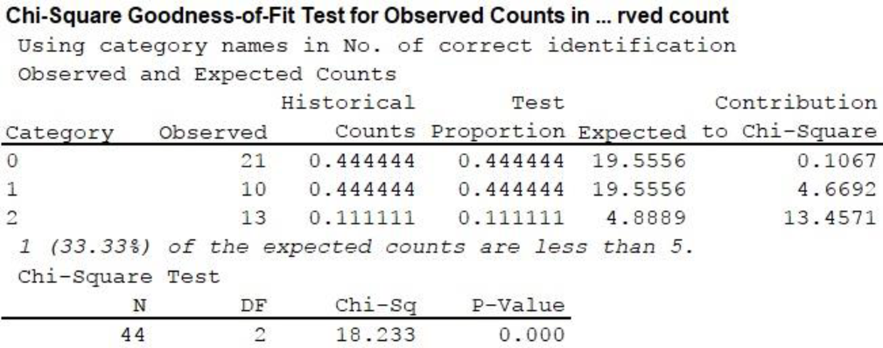
From the output,
8. P-value:
From the MINITAB output,
9. Conclusion:
Decision rule:
- If P-value is less than or equal to the level of significance, reject the null hypothesis.
- Otherwise fail to reject the null hypothesis.
Conclusion:
Here the level of significance is 0.05.
Here, P-value is less than the level of significance.
That is,
Therefore, reject the null hypothesis. Hence, the numbers of correct identifications by the students in this study are significantly different from those that would have been expected by guessing.
Want to see more full solutions like this?
Chapter 12 Solutions
INTRODUCTION TO STATISTICS & DATA ANALYS


- A paper described a survey of 507 undergraduate students at a state university in the southwestern region of the United States. Each student in the sample was classified according to class standing (freshman, sophomore, junior, or senior) and body art category (body piercings only, tattoos only, both tattoos and body piercings, no body art). Use the data in the accompanying table to determine if there is evidence of an association between class standing and response to the body art question. Assume that it is reasonable to regard the sample of students as representative of the students at this university. Use α = 0.01. Freshman Sophomore Junior Senior Body Piercings Only 64 44 20 21 Tattoos Only 7 11 9 17 Both Body Piercings and Tattoos 17 10 7 26 Calculate the test statistic. (Round your answer to two decimal places.) x² = | No Body Art 86 65 46 57 Use technology to calculate the P-value. (Round your answer to four decimal places.) P-value =arrow_forwardIndependent t: The Department of Motor Vehicles (DMV) enlisted the help of a social psychology professor to design a study to see if the attractiveness of the driving instructor affected the performance of young drivers. Thirty 16-year-olds going to take the driving exam were randomly assigned to an attractive or unattractive driving instructor. For 20 of the drivers, the instructor was very attractive; for the other 10 drivers, the instructor was rated as being very unattractive. A panel of judges rated the performance of the two groups, and the mean performance ratings for the 16-year-olds with attractive instructors was 4.3 (S = .86) and with unattractive instructors, the mean was 5.4 (S = 1.30). Using the .05 significance level, did the attractiveness levels of the driving instructor affect driving performance? Use the five steps of hypothesis testing. Sketch the distributions involved. Figure the effect size. Interpret your result placing it back into the context of the…arrow_forward
 Holt Mcdougal Larson Pre-algebra: Student Edition...AlgebraISBN:9780547587776Author:HOLT MCDOUGALPublisher:HOLT MCDOUGAL
 Calculus For The Life SciencesCalculusISBN:9780321964038Author:GREENWELL, Raymond N., RITCHEY, Nathan P., Lial, Margaret L.Publisher:Pearson Addison Wesley,
 Glencoe Algebra 1, Student Edition, 9780079039897...AlgebraISBN:9780079039897Author:CarterPublisher:McGraw Hill