
Concept explainers
Videos
To check: Whether there is sufficient evidence to conclude a difference in means.
To perform: The appropriate test to find out where the difference in means if there is sufficient evidence to conclude a difference in means
Answer to Problem 15CQ
Yes, there is sufficient evidence to conclude a difference in means.
There is significant difference between the means “Asia and Europe” and “Asia and Africa”.
Explanation of Solution
Given info:
The table shows the particulate matter for prominent cities of three continents. The level of significance is 0.05.
Calculation:
The hypotheses are given below:
Null hypothesis:
Alternative hypothesis:
Here, at least one mean is different from the others is tested. Hence, the claim is that, at least one mean is different from the others.
The level of significance is 0.05. The number of samples k is 3, the sample sizes
The degrees of freedom are
Where
Substitute 3 for k in
Substitute 11 for N and 3 for k in
Critical value:
The critical F-value is obtained using the Table H: The F-Distribution with the level of significance
Procedure:
- Locate 8 in the degrees of freedom, denominator row of the Table H.
- Obtain the value in the corresponding degrees of freedom, numerator column below 2.
That is, the critical value is 4.46.
Rejection region:
The null hypothesis would be rejected if
Software procedure:
Step-by-step procedure to obtain thetest statistic using the MINITAB software:
- Choose Stat > ANOVA > One-Way.
- In Response, enter the Gasoline prices.
- In Factor, enter the Factor.
- Click OK.
Output using the MINITAB software is given below:
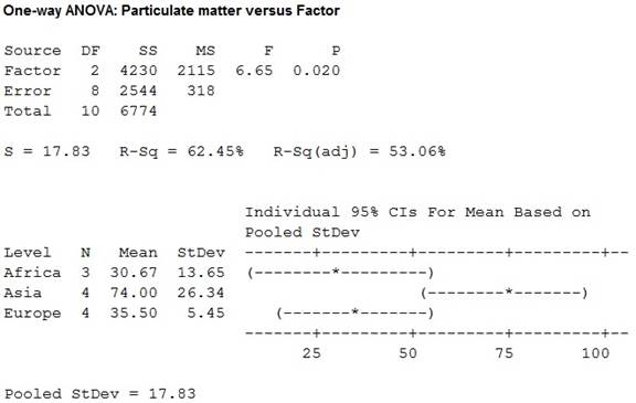
From the MINITAB output, the test value F is 6.65.
Conclusion:
From the results, the test value is 6.65.
Here, the F-statistic value is greater than the critical value.
That is,
Thus, it can be concluding that, the null hypothesis is rejected.
Hence, the result concludes that, there is sufficient evidence to conclude a difference in means.
Consider,
Step-by-step procedure to obtain the test mean and standard deviation using the MINITAB software:
- Choose Stat > Basic Statistics > Display Descriptive Statistics.
- In Variables enter the columns Asia, Europe and Africa.
- Choose option statistics, and select Mean, Variance and N total.
- Click OK.
Output using the MINITAB software is given below:
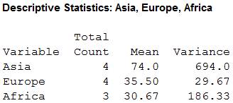
The sample sizes
The means are
The sample variances are
Here, the samples of sizes of three states are not equal. So, the test used here is Scheffe test.
Tukey test:
Critical value:
The formula for critical value F1 for the Scheffe test is,
Here, the critical value of F test is 4.46.
Substitute 4.46 for critical value is of F and 2 for k-1 in
Comparison of the means:
The formula for finding
That is,
Comparison between the means
The hypotheses are given below:
Null hypothesis:
Alternative hypothesis:
Rejection region:
The null hypothesis would be rejected if absolute value greater than the critical value.
The formula for comparing the means
Substitute 74.0 and 35.50 for
Thus, the value of
Conclusion:
The value of
Here, the value of
That is,
Thus, the null hypothesis is rejected.
Hence, there is significant difference between the means
Comparison between the means
The hypotheses are given below:
Null hypothesis:
Alternative hypothesis:
Rejection region:
The null hypothesis would be rejected if absolute value greater than the critical value.
The formula for comparing the means
Substitute 74.0 and 30.67 for
Thus, the value of
Conclusion:
The value of
Here, the value of
That is,
Thus, the null hypothesis is rejected.
Hence, there is significant difference between the means
Comparison between the means
The hypotheses are given below:
Null hypothesis:
Alternative hypothesis:
Rejection region:
The null hypothesis would be rejected if absolute value greater than the critical value.
The formula for comparing the means
Substitute 35.50 and 30.67 for
Thus, the value of
Conclusion:
The value of
Here, the value of
That is,
Thus, the null hypothesis is not rejected.
Hence, there is no significant difference between the means
Justification:
Here, there is significant difference between the means
Want to see more full solutions like this?
Chapter 12 Solutions
Bluman, Elementary Statistics: A Step By Step Approach, © 2015, 9e, Student Edition (reinforced Binding) (a/p Statistics)


- Exhibit 9-5 n = 16 HO: u z 80 x = 75.607 Ha: µ < 80 o = 8.246 Assume the population is normally distributed. 4. Refer to Exhibit 9-5. The p-value is equal to .0332 .9834 -.0166 .0166arrow_forwardA die was rolled 360 times and the results were: No. of Spots (outcomes) Frequency 1 54 2 70 3 58 4 62 5 50 6 66 Is the die balanced at a = 0.05? Determine the tabular value. OA. 18.5476 OB. 11.0705 O C. 12.5916 OD. 16.74arrow_forwardShortleaf Pines. The ability to estimate the volume of a tree based on a simple measurement, such as the diameter of the tree, is important to the lumber industry, ecologists, and conservationists. Data on volume, in cubic feet, and diameter at breast height, in inches, for 70 shortleaf pines was reported in C. Bruce and F. X. Schumacher’s Forest Mensuration (New York: McGraw-Hill, 1935) and analyzed by A. C. Akinson in the article “Transforming Both Sides of a Tree” (The American Statistician, Vol. 48, pp. 307–312). The data are provided on the WeissStats site. a. obtain and interpret the standard error of the estimate. b. obtain a residual plot and a normal probability plot of the residuals. c. decide whether you can reasonably consider Assumptions 1–3 for regression inferences met by the two variables under consideration.arrow_forward
- Everest auto industry produces bearing for Mahindra Motor Corporation. The precision of radius of bearing is very important for its successful functioning. To check the variability in the bearing radius, the company randomly selected ten bearings and measured the radius, the result of which is as shown in the table below. #no Nominal radius (cm) #no Nominal radius (cm) 1 2.70 6 2.59 2 2.65 7 2.73 3 2.75 8 2.64 4 2.55 9 2.88 5 2.76 10 2.83 Calculate the sample standard deviation for the above data. Construct a box plot and check whether there is any outlier data in the data distribution. Based on the comparison between the mean and the quartile, identify the shape of the data distribution. Calculate the 65th percentile and interpret the result. What is the range of the data distribution? Explain its meaning.arrow_forwardAn experiment was conducted to study the extrusion process of biodegradable packaging foam. Two of the factors considered for their effect on the foam diameter (mm) were the die temperature(145°C vs.155°C) and the die diameter (3 mm vs. 4 mm). The results are in the accompanying data table. The question are attached in a photoarrow_forward2. The level of dissolved oxygen in a river is an important indicator of the water's ability to support aquatic life. You collect water samples at 15 randomly chosen locations along a stream and measure the dissolved oxygen. Here are your results in milligrams per liter. 4.53 5.04 3.29 5.23 4.13 5.50 4.83 4.40 5.42 6.38 4.01 4.66 2.87 5.73 5.55 Construct and interpret a 95% confidence interval to estimate the mean dissolved oxygen level in the stream.arrow_forward
- Determine and ox from the given parameters of the population and sample size. μ = 44, o = 10, n = 32 ox= (Round to three decimal places as needed.)arrow_forwardIdentify if the quantity reported is a Parameter or a Statistic: 1. After taking the first exam, 15 of Prof. Kish's students dropped the class. 2. A sample of 120 employees of a company is selected, and the average age is found to be 37 years. 3. The average length of 15 bolts taken from a lot of 50 is 3.05 cm. 4. After interviewing all of John’s employees, a researcher found that theaverage time the workers report late for work is 30 minutes. 5. A consumer magazine reports the air quality as quantified by the degree of staleness measured from 175 of 1000 domestic flights. 6. The average amount of time spent in a day by Mr. John’s students in their online classes is 4 hrs. and 25 minutes. 7. The annual family income of a sample of 210 families of a small town isPhp327,530.8. The number of defective items taken from a randomly selected batch in a production process is 3. 9. The average number of online purchases made in a month by SLU teaching employees is 3.5. 10. The average number of…arrow_forward8. An entrepreneur wanted to assess the quality of eggs produced by his subcontractors. He measured the weight (Y in g) of each egg in a selected pen as well as its circumference (X, in cm) to obtain the size. Define the population of the study.arrow_forward
- Artificial hip joints consist of ball and socket. As the joint wears, the ball (head) becomes rough Investigators performed wear tests on metal artificial hip joints. Joints with several different diameters were tested. The Following table presents measurements of head roughness (in nanometers). Diameter Head Roughness 16 0.83 2.25 0.40 2.78 3.23 28 2.72 2.48 3.80 36 6.49 5.32 4.59 a. Because the design is unbalanced, check that the assumption of equal variances is by showing that the largest sample standard deviation is less than twice as large as the smallest one. b. Construct an ANOVA table. c. Can you conclude that the mean roughness varies with diameter? Use the a=0.01 level of significance.arrow_forwardWhat could be the resulting cross section?arrow_forwardExhibit 10-11An insurance company selected samples of clients under 18 years of age and over 18 and recorded the number of accidents they had in the previous year. The results are shown below. Under Age 18 Over Age 18 n1 = 500 n2 = 600 Number of accidents = 180 Number of accidents = 150 We are interested in determining if the accident proportions differ between the two age groups. Refer to Exhibit 10.11. The p-value is _____. less than .001 more than .10 .0228 .3arrow_forward
 Holt Mcdougal Larson Pre-algebra: Student Edition...AlgebraISBN:9780547587776Author:HOLT MCDOUGALPublisher:HOLT MCDOUGAL
 Glencoe Algebra 1, Student Edition, 9780079039897...AlgebraISBN:9780079039897Author:CarterPublisher:McGraw Hill
 Algebra & Trigonometry with Analytic GeometryAlgebraISBN:9781133382119Author:SwokowskiPublisher:Cengage