
Concept explainers
Videos
(a)
To construct a dot plot of the difference (Standing minus blocks) in
(a)
Explanation of Solution
Firstly, let us find the difference between the time with blocks and time in standing start for each sprinter, i.e.
| Sprinter | With Blocks | Standing Blocks | Difference |
| 1 | 6.12 | 6.38 | -0.26 |
| 2 | 6.42 | 6.52 | -0.1 |
| 3 | 5.98 | 6.09 | -0.11 |
| 4 | 6.8 | 6.72 | 0.08 |
| 5 | 5.73 | 5.98 | -0.25 |
| 6 | 6.04 | 6.27 | -0.23 |
| 7 | 6.55 | 6.71 | -0.16 |
| 8 | 6.78 | 6.8 | -0.02 |
Now we will create a dot plot as:
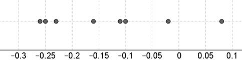
We note that 7 out of 8 dots lie to the left of zero, which indicates that most of the differences are negative and thus that most of the times blocks are less than the times in standing start.
This then implies that the graph suggests that starting blocks are helpful and reduce time. Thus, the graph suggest that the starting blocks are helpful.
(b)
To calculate the mean difference and the standard deviation of the differences and explain why mean differences gives some evidence that the starting blocks are equal.
(b)
Answer to Problem R10.7RE
The mean is
The standard deviation is
Explanation of Solution
As in part (a), we have find the difference between the time and blocks in starting start for each sprinter, we have,
| Sprinter | With Blocks | Standing Blocks | Difference |
| 1 | 6.12 | 6.38 | -0.26 |
| 2 | 6.42 | 6.52 | -0.1 |
| 3 | 5.98 | 6.09 | -0.11 |
| 4 | 6.8 | 6.72 | 0.08 |
| 5 | 5.73 | 5.98 | -0.25 |
| 6 | 6.04 | 6.27 | -0.23 |
| 7 | 6.55 | 6.71 | -0.16 |
| 8 | 6.78 | 6.8 | -0.02 |
The mean of the difference will be as:
Thus the mean is
The standard deviation is the square root of the variance then,
The standard deviation is
Since the sample mean of the difference
(c)
To find out do the data provide the convincing evidence that sprinters like these runs a faster race when using starting blocks on average or not.
(c)
Answer to Problem R10.7RE
There is convincing evidence that sprinters like these run a faster race when using starting blocks, on average.
Explanation of Solution
It is given in the question that:
Now, from part (b), we know that,
The mean is
Thus, the hypothesis test will be as follows:
Claim given: Mean is lower for with blocks.
The claim is either the null hypothesis or the alternative hypothesis.
Let us calculate the test statistics:
The degree of freedom will be:
The P-values will be:
If the P-value is less than the significance level, reject the null hypothesis:
Thus, we have,
So, we can conclude that there is convincing evidence that sprinters like these run a faster race when using starting blocks, on average.
(d)
To construct and interpret
(d)
Answer to Problem R10.7RE
The confidence interval is
We are
Explanation of Solution
It is given in the question that:
Now, from part (b), we know that,
The mean is
The degree of freedom will be:
So, the t -value will be:
So, the margin of error will be:
Then the confidence interval will be calculated as:
Thus, we are
The confidence interval gives more information than the hypothesis test because the confidence interval gives a range of possible values for the mean difference while the hypothesis test only tests a claim about one single value for the mean difference.
Chapter 10 Solutions
PRACTICE OF STATISTICS F/AP EXAM
Additional Math Textbook Solutions
STATS:DATA+MODELS-W/DVD
Basic Business Statistics, Student Value Edition (13th Edition)
Introductory Statistics
Statistics for Business and Economics (13th Edition)
Elementary Statistics: Picturing the World (6th Edition)


 MATLAB: An Introduction with ApplicationsStatisticsISBN:9781119256830Author:Amos GilatPublisher:John Wiley & Sons Inc
 Probability and Statistics for Engineering and th...StatisticsISBN:9781305251809Author:Jay L. DevorePublisher:Cengage Learning
 Statistics for The Behavioral Sciences (MindTap C...StatisticsISBN:9781305504912Author:Frederick J Gravetter, Larry B. WallnauPublisher:Cengage Learning
 Elementary Statistics: Picturing the World (7th E...StatisticsISBN:9780134683416Author:Ron Larson, Betsy FarberPublisher:PEARSON
 The Basic Practice of StatisticsStatisticsISBN:9781319042578Author:David S. Moore, William I. Notz, Michael A. FlignerPublisher:W. H. Freeman
 Introduction to the Practice of StatisticsStatisticsISBN:9781319013387Author:David S. Moore, George P. McCabe, Bruce A. CraigPublisher:W. H. Freeman