
Concept explainers
Videos
a.
Construct a time series plot for temperature using the given data.
Comment on the pattern of obtained time series plot.
a.
Answer to Problem 82SE
Output obtained from MINITAB is given below:
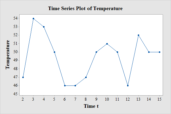
The obtained time series plot represents a cyclic pattern of temperature.
Explanation of Solution
Given info:
The data represents the observed value of response variable x at time t. The observed values are
Calculation:
Software Procedure:
Step-by-step procedure to draw the time series plot for temperature using the MINITAB software:
- Choose Graph > Time Series Plot.
- Choose Simple, and then click OK.
- In Series, enter the column of Temperature.
- Click OK.
Observation:
Time series plot shows that the highest temperature is at time 3 and the lowest temperature is at time 6 and 7. From the graph it can be concluded that temperature oscillates with the change in time. Overall the plot represents a cyclic pattern of temperature.
b.
Find the smoothed value
b.
Answer to Problem 82SE
Smoothed values
| Time t | ||
| 2 | 47 | 47 |
| 3 | 54 | 47.7 |
| 4 | 53 | 48.2 |
| 5 | 50 | 48.4 |
| 6 | 46 | 48.2 |
| 7 | 46 | 48 |
| 8 | 47 | 47.9 |
| 9 | 50 | 48.1 |
| 10 | 51 | 48.4 |
| 11 | 50 | 48.5 |
| 12 | 46 | 48.3 |
| 13 | 52 | 48.6 |
| 14 | 50 | 48.8 |
| 15 | 50 | 48.9 |
Smoothed values
| Time t | ||
| 2 | 47 | 47 |
| 3 | 54 | 50.5 |
| 4 | 53 | 51.8 |
| 5 | 50 | 50.9 |
| 6 | 46 | 48.4 |
| 7 | 46 | 47.2 |
| 8 | 47 | 47.1 |
| 9 | 50 | 48.6 |
| 10 | 51 | 49.8 |
| 11 | 50 | 49.9 |
| 12 | 46 | 47.9 |
| 13 | 52 | 50 |
| 14 | 50 | 50 |
| 15 | 50 | 50 |
Explanation of Solution
Calculation:
The exponential smoothing equation is
Smoothed values
Here, to calculate the smoothed value
That is,
Moreover, it is given that
Hence, the smoothed value
Thus, the smoothed value at time 2 is
The smoothed value
Thus, the smoothed value at time 3 is
Similarly, smoothed values for the remaining times are given below:
| Time t | ||
| 2 | 47 | 47 |
| 3 | 54 | 47.7 |
| 4 | 53 | 48.2 |
| 5 | 50 | 48.4 |
| 6 | 46 | 48.2 |
| 7 | 46 | 48 |
| 8 | 47 | 47.9 |
| 9 | 50 | 48.1 |
| 10 | 51 | 48.4 |
| 11 | 50 | 48.5 |
| 12 | 46 | 48.3 |
| 13 | 52 | 48.6 |
| 14 | 50 | 48.8 |
| 15 | 50 | 48.9 |
Smoothed values
Here, to calculate the smoothed value
That is,
Moreover, it is given that
Hence, the smoothed value
Thus, the smoothed value at time 2 is
The smoothed value
Thus, the smoothed value at time 3 is
Similarly, smoothed values for the remaining times are given below:
| Time t | ||
| 2 | 47 | 47 |
| 3 | 54 | 50.5 |
| 4 | 53 | 51.8 |
| 5 | 50 | 50.9 |
| 6 | 46 | 48.4 |
| 7 | 46 | 47.2 |
| 8 | 47 | 47.1 |
| 9 | 50 | 48.6 |
| 10 | 51 | 49.8 |
| 11 | 50 | 49.9 |
| 12 | 46 | 47.9 |
| 13 | 52 | 50 |
| 14 | 50 | 50 |
| 15 | 50 | 50 |
c.
Find the number of values of
Find the change in the coefficient of
c.
Answer to Problem 82SE
The value of
The coefficient on
Explanation of Solution
Calculation:
The exponential smoothing equation is
Substituting the value,
Substituting the value,
Continuing the same computational procedure till the value of
Now, the equation reduces as follows:
The value of
Now, the exponential smoothing equation
Here, from the above obtained equation it is seen that the value of
Here, form the equation it can be said that the coefficient of
Moreover, the smoothing constant
That is,
Hence the value of
Therefore, the coefficient on
c.
Explain the sensitivity of the initialization of
c.
Answer to Problem 82SE
The smoothed series
Explanation of Solution
Calculation:
From part (c), the exponential smoothing equation is,
The substitution of of
Here, form the equation it can be said that the coefficient of
Moreover, the smoothing constant
That is,
Hence the value of
Therefore, the smoothed series
Want to see more full solutions like this?
Chapter 1 Solutions
Probability and Statistics for Engineering and the Sciences


- Clint, obviously not in college, sleeps an average of 8 hours per night with a standard deviation of 15 minutes. What's the chance of him sleeping between 7.5 and 8.5 hours on any given night? 0-(7-0) 200 91109s and doiw $20 (8-0) mol 8520 slang $199 galbrog seam side pide & D (newid se od poyesvig as PELEO PER AFTE editiw noudab temand van Czarrow_forwardTimes to complete a statistics exam have a normal distribution with a mean of 40 minutes and standard deviation of 6 minutes. Deshawn's time comes in at the 90th percentile. What percentage of the students are still working on their exams when Deshawn leaves?arrow_forwardSuppose that the weights of cereal boxes have a normal distribution with a mean of 20 ounces and standard deviation of half an ounce. A box that has a standard score of o weighs how much? syed by ilog ni 21arrow_forward
- Bob scores 80 on both his math exam (which has a mean of 70 and standard deviation of 10) and his English exam (which has a mean of 85 and standard deviation of 5). Find and interpret Bob's Z-scores on both exams to let him know which exam (if either) he did bet- ter on. Don't, however, let his parents know; let them think he's just as good at both subjects. algas 70) sering digarrow_forwardSue's math class exam has a mean of 70 with a standard deviation of 5. Her standard score is-2. What's her original exam score?arrow_forwardClint sleeps an average of 8 hours per night with a standard deviation of 15 minutes. What's the chance he will sleep less than 7.5 hours tonight? nut bow visarrow_forward
- Suppose that your score on an exam is directly at the mean. What's your standard score?arrow_forwardOne state's annual rainfall has a normal dis- tribution with a mean of 100 inches and standard deviation of 25 inches. Suppose that corn grows best when the annual rainfall is between 100 and 150 inches. What's the chance of achieving this amount of rainfall? wved now of sociarrow_forward13 Suppose that your exam score has a standard score of 0.90. Does this mean that 90 percent of the other exam scores are lower than yours?arrow_forward
- Bob's commuting times to work have a nor- mal distribution with a mean of 45 minutes and standard deviation of 10 minutes. How often does Bob get to work in 30 to 45 minutes?arrow_forwardBob's commuting times to work have a nor- mal distribution with a mean of 45 minutes and standard deviation of 10 minutes. a. What percentage of the time does Bob get to work in 30 minutes or less? b. Bob's workday starts at 9 a.m. If he leaves at 8 a.m., how often is he late?arrow_forwardSuppose that you want to put fat Fido on a weight-loss program. Before the program, his weight had a standard score of +2 com- pared to dogs of his breed/age, and after the program, his weight has a standard score of -2. His weight before the program was 150 pounds, and the standard deviation for the breed is 5 pounds. a. What's the mean weight for Fido's breed/ age? b. What's his weight after the weight-loss program?arrow_forward
 College AlgebraAlgebraISBN:9781305115545Author:James Stewart, Lothar Redlin, Saleem WatsonPublisher:Cengage Learning
 Glencoe Algebra 1, Student Edition, 9780079039897...AlgebraISBN:9780079039897Author:CarterPublisher:McGraw Hill
 Algebra and Trigonometry (MindTap Course List)AlgebraISBN:9781305071742Author:James Stewart, Lothar Redlin, Saleem WatsonPublisher:Cengage Learning
 Trigonometry (MindTap Course List)TrigonometryISBN:9781337278461Author:Ron LarsonPublisher:Cengage Learning
 Big Ideas Math A Bridge To Success Algebra 1: Stu...AlgebraISBN:9781680331141Author:HOUGHTON MIFFLIN HARCOURTPublisher:Houghton Mifflin Harcourt