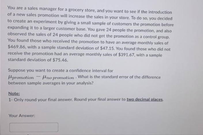
You are a sales manager for a grocery store, and you want to see if the introduction of a new sales promotion will increase the sales in your store. To do so, you decided to create an experiment by giving a small sample of customers the promotion before expanding it to a larger customer base. You gave 24 people the promotion, and also observed the sales of 24 people who did not get the promotion as a control group. You found those who received the promotion to have an average monthly sales of $469.86, with a sample standard deviation of $47.15. You found those who did not receive the promotion had an average monthly sales of $391.67, with a sample standard deviation of $75.46. Suppose you want to create a confidence interval for Hpromotion no promotion What is the standard error of the difference . between sample averages in your analysis? Note: 1- Only round your final answer. Round your final answer to two decimal places. Your Answer:

It is often useful for retailers to determine why their potential customers chose to visit their store. Possible reasons include advertising, advice from a friend, or previous experience. To determine the effect of full-page advertisements in the local newspaper, the owner of an electronic-equipment store asked  randomly selected people who visited the store whether they had seen the ad. He also determined whether the customers had bought anything, and if so, how much they spent. Among the respondents who saw the ad, 49 made an average purchase of $97.38 with a variance of $622. Among the respondents who did not see the ad, 21 made an average purchase of  $92.01 with a variance of $283.3. Can the owner conclude that customers who see the ad spend more than those who do not see the ad (among those who make a purchase) at 5% significance level?     Population:  One Two Multiple       Formula #: Answer  Hypothesis Null H0 : (μ, π, σ², μd, μ1 - μ2, π1- π2, σ₁²…

In 2013, 46% of high school students tried a tobacco product. From a survey of 500 randomly  selected high school students, how likely is it to get a proportion of 0.196 that tried a tobacco product?

As an admissions counselor, I am interested in understanding whether or not there is a difference in stress levels not only between different majors but also between different classes (Freshman v. Seniors). I gather the following data from students from three majors (Psychology, Chemistry, and Engineering), that are in their freshmen or senior years and ask them about their stress levels (scale of 1-10, with lower numbers meaning less stress). Using the data below, test whether there are effects of class, major, or an interaction between them at an alpha of 0.05.    Psychology Chemistry Engineering Freshmen 3, 4, 4, 2, 4 4, 5, 7, 8, 4 5, 7, 7, 8, 5 Senior 4, 5, 5, 3, 5 8, 5, 6, 7, 7 9, 9, 8, 7, 9 Complete the ANOVA summary table below:  Source SS df MS (variance) F MAJOR         CLASS         MAJOR*CLASS         ERROR/RESIDUAL       Nothing here TOTAL     Nothing here Nothing here   What can we conclude?…