Answered: What this particular plot shows about…

Math

Statistics

What this particular plot shows about the model being analysed?

Algebra & Trigonometry with Analytic Geometry

13th Edition

ISBN:9781133382119

Author:Swokowski

Publisher:Swokowski

Chapter1: Fundamental Concepts Of Algebra

Section1.1: Real Numbers

Problem 49E

See similar textbooks

Related questions

Q: In the following problem, check that it is appropriate to use the normal approximation to the…

A: The objective of this question is to determine whether it is appropriate to use the normal…

Q: From the figure below, what is (approximately) the most likely value for the frequency of the mean…

A: The frequency chart of size classes of cockles:The most likely value for the frequency of the mean…

Q: For each item, show ALL calculations. High density lipoprotein (HDL) in healthy males follows a…

Q: ation of 3.1 minutes. Assume the variable is normally distributed. When a customer arrives at the…

A: Let X be the random variable the waiting time to be seated for dinner.Given that,

Q: David's gasoline station offers 4 cents off per gallon if the customer pays in cash and does not use…

A: The question is about discrete probability distribution.Given :Proportion of all customers who pay…

Q: The heights of 1000 students are approximately normally distributed with a mean of 173.8 centimeters…

A: The question is about sampling distribution.Given :Population mean height of students ( ) = 173.8…

Q: Construct a 95% confidence interval to estimate the population mean when x = 65 and s = 14.5 for the…

A: Sample mean=65Standard deviation =14.5

Q: A new over-the-counter medicine to treat a sore throat is to be tested for effectiveness. The makers…

A: The objective of this question is to determine the 95% confidence interval for the difference in…

Q: The predictive distribution pynewy) for a new observation Ynew takes into account the posterior…

A: Given observed data y, the predictive distribution for a new observation y_(new) can be expressed as…

Q: 4. Prove that var(ax + bY) = a² var(X) + b² var (Y) + 2ab cov (Y, X)

A: Let X and Y be two random variables

Q: 1) We are creating a new card game with a new deck. Unlike the normal deck that has 13 ranks (Ace…

A: Given ,The deck will be made up of the following: Each card will have : i) one rank from 1 to 17…

Q: In the following table, price of a used car is given in terms of the percentage of the car's…

A: The objective of this question is to find the best linear fit to the given data that minimizes the…

Q: Consider the following two equations. i. y₁ = 4x 1.2 ii. y = 1 + 3x + 1.6x 2 Compute the values of y…

A: The two equations are:(i) yi=4x1.2(ii) yi=1+3xi+1.6xi2The objective is to calculate yi for the given…

Q: Q10.5

A: (a) As the confidence level increases, the interval becomes wider.(b) As the sample size increases,…

Q: Find out the required runway length for the airport of reference code 4D located at 450m above mean…

A: The objective of the question is to calculate the required runway length for an airport of reference…

Q: In the panel regression analysis of beer taxes on traffic deaths, the estimation period is 1982-1988…

A: To test for the significance of time fixed effects at the 1% level in a panel regression analysis,…

Q: +3 You are given that +980 = 125 Calculate Var[K80]. A 0.87 B 0.90 C 0.93 D 0.96 E 0.99

A: We have givenTherefore,To find:

Q: Q10.2

A: a . To find the point estimate of the true mean salt content ($ \mu $) for frankfurters, you need…

Q: In 2014, the Centers for Disease Control and Prevention (CDC) reported the percentage of people 18…

A: From the provided information,Population proportion (p) = 0.30.Confidence level = 95%The margin of…

Q: Determine the value of z such that the area to the right of z is 0.9906. Round the solution to two…

A: Given ,The area to the right of z is 0.9906 We have to find the value of z

Q: Let Y be uniformly distributed in [0, 1], and X = In(Y+1). Find the cumulative distributionfunction…

A: For any provided value, the CDF tells the possibility that a random variable will be less than or…

Q: The plant-breeding department at a major university developed a new hybrid boysenberry plant called…

A: The objective of the question is to understand the concept of a Type I error in the context of…

Q: K In a certain state, it has been shown that only 54% of the high school graduates who are capable…

A: The objective of this question is to find the probability that, among 10 capable high school…

Q: he truck drivers. How might this data-collection method produce bias in obtaining an estimate of all…

A: Given that,A sticker on the rear bumper is given along with the phone number.This sticker allows…

Q: Maya recently switched her primary doctor to one specializing in caring for elderly patients. On her…

A: The objective of this question is to determine whether the mean systolic blood pressure among…

Q: A random variable x follows Binomial distribution with mean 2 and variance 1.2. Then the value of n…

Q: here is question 9 being posted

A: The decision rule is reject H0 if the test statistic is less than -1.645 or greater than…

Q: Melanie buys a bag of cookies that contains 9 chocolate chip cookies, 7 peanut butter cookies, 8…

A: Note:Hi there! Thank you for posting the question. To avoid the plagiarism issues, we have used the…

Q: 1330 1420 1510 1600 1690 1780 1870 Distribution of Prices a What is the approximate percentage of…

A: given graph is

Q: A sample of 1100 computer chips revealed that 25% of the chips fail in the first 1000 hours of their…

A: H0 : p = 0.28Ha : p ≠ 0.28 There is sufficient evidence at the 0.10 significance level to dispute…

Q: 2. Describe the direction and strength of the correlations from the following scatterplots. (Are…

A: Perfect correlation: The correlation is said to be perfect if all the points fall in a straight…

Q: Given the probability distribution below, find the missing value, : -71 0.121 39 y 85…

A: The objective of this question is to find the missing probability value, y, in the given probability…

Q: Using the z-Table, find the exact area of the region associated with the following probability.…

A: We have to find the exact area of the region associated with the probability. P(z>0.52)

Q: Draw a normal distribution for each of the following z-score locations. Then draw a vertical line…

A: If the value of Z-score is negative then say that this is left -tail and if Z-score is positive then…

Q: 6.2 不 Question 3 of 17 This quiz: 17 point(s) possible This question: 1 point(s) possible Submit…

A: The 95% confidence interval for the population mean μ is (60.11,99.89).The margin of error is…

Q: A manufacturing unit has to appoint a committee consisting of 4 people. There are 9 eligible…

A: Given , A manufacturing unit has to appoint a committee consisting of 4 people. ie, There are 9…

Q: pular restaurant is 23.2 minutes, with a dard deviation of 3.1 minutes. Assume the ble is normally…

A: Population mean =23.2Population standard deviation =3.1

Q: Suppose you have access to a database with the variables listed below. Choose two variables you are…

A: The objective of the question is to identify two variables from the given database that may have a…

Q: 3. Approximately 3.6% of all (untreated) Jonathan apples had bitter pit in a study conducted by the…

A: The probability shows how likely an event occurs and it can take any value between 0 and 1.

Q: Under the assumptions of the Simple Linear Regression (SLR) model: a. Show that Cov (B0, 1) = 0.…

A: Using the simple linear regression model We have to show that Cov(β0^,β1^)=-x¯/(σ2/Sxx)And based on…

Q: B Quiz: 6.1 & 6.2 13 Question 15 of 17 This quiz: 17 point(s) possible This question: 1 point(s)…

A: The objective of the question is to understand the concept of a 95% confidence interval and to…

Q: The following graph illustrates 140 120 100 10 20 40 50 60 70 80 X

A: You are given a scatter plot of data on X and Y. You just need to select the appropriate…

Q: Find each of the following probabilities for a normal distribution. (Hint: use the three step method…

A: Given that a distribution is normally distributed We have to find Z > .25Z > -.75Z < 1.20Z…

Q: question 11 response =yes sample size= 200 count for response 114 sample proportion 0.5700…

A: To find the critical value for the given hypothesis test, where the confidence coefficient is 0.95…

Q: In a survey of 500 students, 320 preferred pizza, 150 preferred burgers, and the rest preferred…

A: To find the percentage of students who preferred sandwiches, we need to subtract the number of…

Q: A sample of 1100 computer chips revealed that 67 % of the chips fail in the first 1000 hours of…

A: The objective of this question is to test the null hypothesis that the actual failure rate of the…

Q: (a) The boy first selected a star and then a circle. (b) The boy first selected a circle and then a…

A: Indigenous game played with decoration of 5 stone with decoration 2 circle and 3 star decoration on…

Q: Let X₁, . . ., Xn be a random sample from N(0, 1), 0 = R, find UMVUE of e-? Let X₁, ..., Xn be a…

A: denotes a random sample from the normal distribution .The UMVUE of must be calculated.

Q: In a random sample of 50 Americans five years ago (Group 1), the average credit card debt was…

A: Given ,Significance level , 0.01For group 1 : $5798$1154sample size, 50For group 2 :…

Q: A batsman played with an average of 78 runs per match in first 28 matches. In the next 14 matches,…

Question

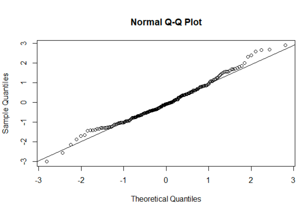
The CSV file modeldata.csv contains 200 observations of 4 explanatory variables (x1, x2, x3, x4) and a response variable (y). A multiple linear regression model is built in R using the following code,

> modeldata <- read.csv("modeldata.csv") > x1 <- modeldata$x1 > x2 <- modeldata$x2 > x3 <- modeldata$x3 > x4 <- modeldata$x4 > y <- modeldata$y > model <- lm(y~x1+x2+x3+x4)

Question: What this particular plot shows about the model being analysed?