-week period (1 January 2022 – 14 January 2022). Whilst this is not a particularly large contract for OBL, the Board of Directors is hopeful that significantly more work will follow.   The data relating to the production of each component is as follows:

Survey of Accounting (Accounting I)
8th Edition
ISBN:9781305961883
Author:Carl Warren
Publisher:Carl Warren
Chapter15: Capital Investment Analysis
Section: Chapter Questions
Problem 15.5.3MBA
icon
Related questions
Question

Orange Box Limited (‘OBL’) is a small specialist manufacturer of specialist electronic components, selling much of its output to both civil and military aircraft manufacturers.


It is 1 December 2021 and one of these aircraft manufacturers has offered a contract to OBL for the supply of 200 identical components over a two-week period (1 January 2022 – 14 January 2022). Whilst this is not a particularly large contract for OBL, the Board of Directors is hopeful that significantly more work will follow.


The data relating to the production of each component is as follows:


Material requirements


3 kg material X1

Material X1 is in continuous use by the company. 500 kg are currently held in inventory. These materials were purchased for £5.15/kg but it is known that future purchases will cost

£5.50/kg


2 kg material X2

600 kg of material X2 are held in inventory. The original cost of this material was £3.55/kg but, as the material has not been required for the last two years, it has been written down to its scrap value of £1.50/kg. The only foreseeable alternative use is as a substitute for material X4 (in current continuous use) but this would involve further processing costs of

£2.50/kg. The current cost of material X4 is £4.50/kg.


1 component JKL

There are 500 components of JKL in inventory. These originally cost £50 each but have no other use in OBL.


Labour requirements


Each component would require five hours of skilled labour and five hours of semi-skilled labour.


  • Skilled labour is currently paid £15/hour. Replacement workers would, however, require to be hired at a rate of £14/hour for the work which would otherwise be done by the skilled


  • The current rate for semi-skilled work is £12/hour and OBL will require to hire these workers as the company currently has no semi-skilled


There is also a requirement for two weeks of time for a specialist engineer who is paid a weekly salary of £1,000 for working a 40-hour week. She would be required to be removed from another contract (Contract ZZZ) which generates a contribution of £5 per engineer hour. There are no other engineers available to continue with Contract ZZZ if she is taken off this contract. This would mean that OBL would miss its contractual deadline on Contract ZZZ (14 January 2022) by two weeks and would require to pay a one-off penalty of £2,500. As there is no other work currently scheduled for the engineer after 14 January 2022, it will not be a problem for OBL to complete Contract ZZZ at this point.


The supervisor who will be responsible for the new contract with the aircraft manufacturer should it be won, is paid an annual salary of £52,000. She has the capacity within her existing workload to supervise this new contract. It is OBL corporate policy to allocate supervisor salary costs to individual contracts on the basis of time spent.


Overheads


OBL absorb overheads by a machine hour rate, currently £22/hour, of which £8 is for variable overheads and £14 for fixed overheads. If this contract is undertaken, it is estimated that fixed costs will increase for the duration of the contract by £5,500. Spare machine capacity is available and each component would require four machine hours.


Other information


The CEO of OBL required to hold a meeting with the CEO of the aircraft manufacturer in November 2021 to discuss the proposed contract requirements. The costs of this meeting were £500. A contract price of £225 per component was suggested by the CEO of the aircraft manufacturer after the meeting.


Required:


  1. Advise the Board of Directors whether the contract should be accepted. Support your conclusion with appropriate figures and explanations. Show all


  1. Comment on four factors that the Board of Directors ought to consider and which may influence its final

(Five maximum word limit)
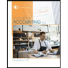
Present Value and Annuity Tables
Table I: Present value tables
Present value of I = (1 + r)¯"
Present value of I = (1 + r)¯n
r = discount rate
r= discount rate
n = number of periods
Periods 1%
2%
3%
4%
5%
6%
7%
8%
9%
10%
Periods I1%
1 2%
13%
14%
1%
16%
17%
18%
19%
20%
0.990 0.980 0.971
0.962 0.952 0.943 0.935 0.926 0.917 0.909
0.901 0.893 0.885 0.877 0.870 0.862 0.855 0.847 0.840 0.833
0.980 0.961
0.943
0.925
0.907
0.890 0.873 0.857
0.842 0.826
2
0.812 0.797 0.783 0.769 0.756 0.743 0.731 0.718 0.706 0.694
3
0.971
0.942
0.915 0.889 0.864 0.840 0.816 0.794 0.772 0.751
3
0.731
0.712 0.693 0.675 0.658 0.641 0.624 0.609 0.593 0.579
4
0.961 0.924 0.888 0.855 0.823
0.792 0.763 0.735 0.708 0.683
4
0.659 0.636 0.613 0.592 0.572 0.552 0.534 0.516 0.499 0.482
0.951 0.906
0.863
0.822 0.784 0.747
0.713
0.681
0.650
0.621
5
0.593 0.567 0.543 0.519 0.497 0.476 0.456 0.437 0.419 0.402
6
0.942 0.888 0.837 0.790 0.746 0.705
0.666 0.630 0.596
0.564
6
0.535 0.507 0.480 0.456 0.432 0.410 0.390 0.370 0.352 0.335
7
0.933 0.871 0.813
0.760 0.71|
0.665 0.623
0.583 0.547 0.513
7
0.482 0.452 0.425 0.400 0.376 0.354 0.333 0.314 0.296 0.279
8
0.923 0.853 0.789 0.731
0.677 0.627 0.582 0.540 0.502 0.467
8.
0.434 0.404 0.376 0.351 0.327 0.305 0.285 0.266 0.249 0.233
9
0.914 0.837 0.766 0.703 0.645 0.592 0.544 0.500 0.460 0.424
9
0.391
0.361 0.333 0.308 0.284 0.263 0.243 0.225 0.209 0.194
10
0.905 0.820 0.744 0.676 0.614 0.558 0.508 0.463 0.422
0.386
10
0.352 0.322 0.295 0.270 0.247 0.227 0.208 0.191 0.176 0.162
0.896 0.804
0.722
0.650 0.585 0.527 0.475 0.429 0.388
0.350
||
0.317 0.287 0.261 0.237 0.215 0.195 0.178 0.162 0.148 0.135
12
0.887 0.788 0.701
0.625 0.557 0.497 0.444 0.397 0.356 0.319
12
0.286 0.257 0.231 0.208 0.187 0.168 0.152 0.137 0.124 0.112
13
0.879 0.773 0.681
0.601
0.530 0.469 0.415 0.368
0.326 0.290
13
0.258 0.229 0.204 0.182 0.163 0.145 0.130 0.116 0.104 0.093
14
0.870 0.758 0.661
0.577 0.505 0.442 0.388 0.340 0.299 0.263
14
0.232 0.205 0.181
0.160 0.141
0.125 0.11| 0.099 0.088 0.078
15
0.861
0.743 0.642
0.555
0.481
0.417 0.362
0.315 0.275 0.239
15
0.209 0.183 0.160 0.140 0.123 0.108 0.095 0.084 0.074 0.065
16
0.853 0.728 0.623
0.534
0.458 0.394 0.339 0.292 0.252 0.218
16
0.188 0.163 0.141 0.123 0.107 0.093 0.081 0.071 0.062 0.054
17
0.844 0.714 0.605 0.513 0.436 0.371 0.317 0.270 0.231
0.198
17
0.170 0.146 0.125 0.108 0.093 0.080 0.069 0.060 0.052 0.045
18
0.836 0.700 0.587 0.494 0.416 0.350 0.296 0.250 0.212 0.180
18
0.153 0.130 0.1|I
0.095 0.081
0.069 0.059 0.051
0.044 0.038
19
0.828 0.686
0.570 0.475
0.396 0.331
0.277
0.232
0.194 0.164
19
0.138 0.116 0.098 0.083 0.070 0.060 0.051
0.043 0.037 0.031
20
0.820 0.673
0.554 0.456 0.377 0.312 0.258 0.215 0.178 0.149
20
0.124 0.104 0.087 0.073 0.061 0.051 0.043
0.037 0.031
0.026
Table 2: Annuity tables
Present value of an annuity of I =
1-(1+r)-n
1-(1-r)-n
Present value of an annuity of =
r = discount rate
r = discount rate
n = number of periods
Periods I1%
12%
13%
14%
15%
16%
17%
18%
19%
20%
Periods 1%
2%
3%
4%
5%
6%
7%
8%
9%
10%
0.901 0.893 0.885 0.877 0.870 0.862 0.855 0.847 0.840 0.833
0.990
0.980
0.971
0.962
0.952
0.943
0.935
0.926 0.917 0.909
2
1.713 1.690 1.668 1.647 1.626 1.605 1.585 1.566 1.547 1.528
2
1.970
1.942
1.913
1.886
1.859
1.833
1.808
1.783 1.759 1.736
3
2.444 2.402 2.361 2.322 2.283 2.246 2.210 2.174 2.140 2.106
3
2.941
2.884
2.829
2.775
2.723
2.673
2.624
2.577 2.531 2.487
4
3.902
3.808
3.717
3.630
3.546
3.465
3.387
3.312 3.240 3.170
4
3.102 3.037 2.974 2.914 2.855 2.798 2.743 2.690 2.639 2.589
4.853
4.713
4.580
4.452
4.329
4.212
4. 100
3.993 3.890 3.791
3.696 3.605 3.517 3.433 3.352 3.274 3.199 3.127 3.058 2.991
6
5.795
5.601
5.417
5.242
5.076
4.917
4.767
4.623 4.486 4.355
6
4.231 4.111 3.998 3.889 3.784 3.685 3.589 3.498 3.410 3.326
6.728
6.472
6.230
6.002
5.786
5.582
5.389
5.206 5.033 4.868
7
4.712 4.564 4.423 4.288 4.160 4.039 3.922 3.812 3.706 3.605
8
7.652
7.325
7.020
6.733
6.463
6.210
5.97|
5.747 5.535 5.335
8
5.146 4.968 4.799 4.639 4.487 4.344 4.207 4.078 3.954 3.837
9
8.566
8.162
7.786
7.435
7.108
6.802
6.515
6.247 5.995 5.759
5.537 5.328 5.132 4.946 4.772 4.607
4.45I
4.303 4.163 4.031
10
9.471
8.983
8.530
8.111
7.722
7.360
7.024
6.710 6.418 6.145
10
5.889 5.650 5.426 5.216 5.019 4.833 4.659 4.494 4.339 4.192
10.368 9.787
9.253
8.760
8.306
7.887
7.499
7.139 6.805
6.495
||
6.207 5.938 5.687
5.453 5.234 5.029 4.836 4.656 4.486 4.327
12
I1.255 10.575
9.954
9.385
8.863
8.384
7.943
7.536 7.161 6.814
13
12.134 |1.348 10.635 9.986
9.394
8.853
8.358
7.904 7.487 7.103
12
6.492 6.194 5.918 5.660 5.421 5.197 4.988 4.793 4.6||
4.439
14
13.004 12.106 11.296 10.563 9.899
9.295
8.745
8.244 7.786 7.367
13
6.750 6.424 6.122 5.842 5.583 5.342 5.118 4.910 4.715 4.533
15
13.865 12.849
11.938 II.118 10.380 9.712
9. 108
8.559 8.06I 7.606
14
6.982 6.628 6.302 6.002 5.724 5.468 5.229 5.008 4.802 4.61|
16
14.718 13.578 12.561
11.652
10.838 10.106 9.447
8.85 8.313 7.824
15
7.191 6.811 6.462 6.142 5.847 5.575 5.324 5.092 4.876 4.675
17
15.562 14.292 13.166 12.166 I1.274 10.477 9.763
9.122 8.544 8.022
16
7.379 6.974 6.604 6.265 5.954 5.668 5.405 5.162 4.938
4.730
18
16.398 14.992
13.754 12.659 |1.690 10.828 10.059
9.372 8.756 8.201
17
7.549 7.120 6.729
6.373
6.047 5.749 5.475 5.222 4.990 4.775
19
17.226 15.678
14.324 13.134
12.085 11.158 10.336 9.604 8.950 8.365
18
7.702 7.250 6.840 6.467 6.128 5.818 5.534 5.273 5.033 4.812
20
18.046 16.351
14.877 13.590
12.462 |1.47O 10.594
9.818 9.129 8.514
19
7.839 7.366 6.938 6.550 6.198 5.877 5.584 5.316 5.070 4.843
20
7.963 7.469 7.025 6.623 6.259 5.929 5.628 5.353 5.101 4.870
Transcribed Image Text:Present Value and Annuity Tables Table I: Present value tables Present value of I = (1 + r)¯" Present value of I = (1 + r)¯n r = discount rate r= discount rate n = number of periods n = number of periods Periods 1% 2% 3% 4% 5% 6% 7% 8% 9% 10% Periods I1% 1 2% 13% 14% 1% 16% 17% 18% 19% 20% 0.990 0.980 0.971 0.962 0.952 0.943 0.935 0.926 0.917 0.909 0.901 0.893 0.885 0.877 0.870 0.862 0.855 0.847 0.840 0.833 0.980 0.961 0.943 0.925 0.907 0.890 0.873 0.857 0.842 0.826 2 0.812 0.797 0.783 0.769 0.756 0.743 0.731 0.718 0.706 0.694 3 0.971 0.942 0.915 0.889 0.864 0.840 0.816 0.794 0.772 0.751 3 0.731 0.712 0.693 0.675 0.658 0.641 0.624 0.609 0.593 0.579 4 0.961 0.924 0.888 0.855 0.823 0.792 0.763 0.735 0.708 0.683 4 0.659 0.636 0.613 0.592 0.572 0.552 0.534 0.516 0.499 0.482 0.951 0.906 0.863 0.822 0.784 0.747 0.713 0.681 0.650 0.621 5 0.593 0.567 0.543 0.519 0.497 0.476 0.456 0.437 0.419 0.402 6 0.942 0.888 0.837 0.790 0.746 0.705 0.666 0.630 0.596 0.564 6 0.535 0.507 0.480 0.456 0.432 0.410 0.390 0.370 0.352 0.335 7 0.933 0.871 0.813 0.760 0.71| 0.665 0.623 0.583 0.547 0.513 7 0.482 0.452 0.425 0.400 0.376 0.354 0.333 0.314 0.296 0.279 8 0.923 0.853 0.789 0.731 0.677 0.627 0.582 0.540 0.502 0.467 8. 0.434 0.404 0.376 0.351 0.327 0.305 0.285 0.266 0.249 0.233 9 0.914 0.837 0.766 0.703 0.645 0.592 0.544 0.500 0.460 0.424 9 0.391 0.361 0.333 0.308 0.284 0.263 0.243 0.225 0.209 0.194 10 0.905 0.820 0.744 0.676 0.614 0.558 0.508 0.463 0.422 0.386 10 0.352 0.322 0.295 0.270 0.247 0.227 0.208 0.191 0.176 0.162 0.896 0.804 0.722 0.650 0.585 0.527 0.475 0.429 0.388 0.350 || 0.317 0.287 0.261 0.237 0.215 0.195 0.178 0.162 0.148 0.135 12 0.887 0.788 0.701 0.625 0.557 0.497 0.444 0.397 0.356 0.319 12 0.286 0.257 0.231 0.208 0.187 0.168 0.152 0.137 0.124 0.112 13 0.879 0.773 0.681 0.601 0.530 0.469 0.415 0.368 0.326 0.290 13 0.258 0.229 0.204 0.182 0.163 0.145 0.130 0.116 0.104 0.093 14 0.870 0.758 0.661 0.577 0.505 0.442 0.388 0.340 0.299 0.263 14 0.232 0.205 0.181 0.160 0.141 0.125 0.11| 0.099 0.088 0.078 15 0.861 0.743 0.642 0.555 0.481 0.417 0.362 0.315 0.275 0.239 15 0.209 0.183 0.160 0.140 0.123 0.108 0.095 0.084 0.074 0.065 16 0.853 0.728 0.623 0.534 0.458 0.394 0.339 0.292 0.252 0.218 16 0.188 0.163 0.141 0.123 0.107 0.093 0.081 0.071 0.062 0.054 17 0.844 0.714 0.605 0.513 0.436 0.371 0.317 0.270 0.231 0.198 17 0.170 0.146 0.125 0.108 0.093 0.080 0.069 0.060 0.052 0.045 18 0.836 0.700 0.587 0.494 0.416 0.350 0.296 0.250 0.212 0.180 18 0.153 0.130 0.1|I 0.095 0.081 0.069 0.059 0.051 0.044 0.038 19 0.828 0.686 0.570 0.475 0.396 0.331 0.277 0.232 0.194 0.164 19 0.138 0.116 0.098 0.083 0.070 0.060 0.051 0.043 0.037 0.031 20 0.820 0.673 0.554 0.456 0.377 0.312 0.258 0.215 0.178 0.149 20 0.124 0.104 0.087 0.073 0.061 0.051 0.043 0.037 0.031 0.026 Table 2: Annuity tables Present value of an annuity of I = 1-(1+r)-n 1-(1-r)-n Present value of an annuity of = r = discount rate r = discount rate n = number of periods n = number of periods Periods I1% 12% 13% 14% 15% 16% 17% 18% 19% 20% Periods 1% 2% 3% 4% 5% 6% 7% 8% 9% 10% 0.901 0.893 0.885 0.877 0.870 0.862 0.855 0.847 0.840 0.833 0.990 0.980 0.971 0.962 0.952 0.943 0.935 0.926 0.917 0.909 2 1.713 1.690 1.668 1.647 1.626 1.605 1.585 1.566 1.547 1.528 2 1.970 1.942 1.913 1.886 1.859 1.833 1.808 1.783 1.759 1.736 3 2.444 2.402 2.361 2.322 2.283 2.246 2.210 2.174 2.140 2.106 3 2.941 2.884 2.829 2.775 2.723 2.673 2.624 2.577 2.531 2.487 4 3.902 3.808 3.717 3.630 3.546 3.465 3.387 3.312 3.240 3.170 4 3.102 3.037 2.974 2.914 2.855 2.798 2.743 2.690 2.639 2.589 4.853 4.713 4.580 4.452 4.329 4.212 4. 100 3.993 3.890 3.791 3.696 3.605 3.517 3.433 3.352 3.274 3.199 3.127 3.058 2.991 6 5.795 5.601 5.417 5.242 5.076 4.917 4.767 4.623 4.486 4.355 6 4.231 4.111 3.998 3.889 3.784 3.685 3.589 3.498 3.410 3.326 6.728 6.472 6.230 6.002 5.786 5.582 5.389 5.206 5.033 4.868 7 4.712 4.564 4.423 4.288 4.160 4.039 3.922 3.812 3.706 3.605 8 7.652 7.325 7.020 6.733 6.463 6.210 5.97| 5.747 5.535 5.335 8 5.146 4.968 4.799 4.639 4.487 4.344 4.207 4.078 3.954 3.837 9 8.566 8.162 7.786 7.435 7.108 6.802 6.515 6.247 5.995 5.759 5.537 5.328 5.132 4.946 4.772 4.607 4.45I 4.303 4.163 4.031 10 9.471 8.983 8.530 8.111 7.722 7.360 7.024 6.710 6.418 6.145 10 5.889 5.650 5.426 5.216 5.019 4.833 4.659 4.494 4.339 4.192 10.368 9.787 9.253 8.760 8.306 7.887 7.499 7.139 6.805 6.495 || 6.207 5.938 5.687 5.453 5.234 5.029 4.836 4.656 4.486 4.327 12 I1.255 10.575 9.954 9.385 8.863 8.384 7.943 7.536 7.161 6.814 13 12.134 |1.348 10.635 9.986 9.394 8.853 8.358 7.904 7.487 7.103 12 6.492 6.194 5.918 5.660 5.421 5.197 4.988 4.793 4.6|| 4.439 14 13.004 12.106 11.296 10.563 9.899 9.295 8.745 8.244 7.786 7.367 13 6.750 6.424 6.122 5.842 5.583 5.342 5.118 4.910 4.715 4.533 15 13.865 12.849 11.938 II.118 10.380 9.712 9. 108 8.559 8.06I 7.606 14 6.982 6.628 6.302 6.002 5.724 5.468 5.229 5.008 4.802 4.61| 16 14.718 13.578 12.561 11.652 10.838 10.106 9.447 8.85 8.313 7.824 15 7.191 6.811 6.462 6.142 5.847 5.575 5.324 5.092 4.876 4.675 17 15.562 14.292 13.166 12.166 I1.274 10.477 9.763 9.122 8.544 8.022 16 7.379 6.974 6.604 6.265 5.954 5.668 5.405 5.162 4.938 4.730 18 16.398 14.992 13.754 12.659 |1.690 10.828 10.059 9.372 8.756 8.201 17 7.549 7.120 6.729 6.373 6.047 5.749 5.475 5.222 4.990 4.775 19 17.226 15.678 14.324 13.134 12.085 11.158 10.336 9.604 8.950 8.365 18 7.702 7.250 6.840 6.467 6.128 5.818 5.534 5.273 5.033 4.812 20 18.046 16.351 14.877 13.590 12.462 |1.47O 10.594 9.818 9.129 8.514 19 7.839 7.366 6.938 6.550 6.198 5.877 5.584 5.316 5.070 4.843 20 7.963 7.469 7.025 6.623 6.259 5.929 5.628 5.353 5.101 4.870
Financial ratios
Creditors days
Working capital
Cost of capital
Gross margin (%)
Economic order quantity (EOQ)
Cost of equity
Trade payables
Gross profit
x 365
Purchases
× 100
2DC
ke =
Do(1+g)
+ g
Po
Revenue
or
H
Operating margin (%)
Trade creditors
or
Operating profit
x 100
x 365
Cash management (1)
Purchases
ke = R, + B(Rm – R;)
Revenue
If 'Purchases' figure not available, use 'Cost of sales
2NF
Z =
Return on capital employed (%)
Financial gearing (%)
WACC
Cash management (2)
Ve
ke:
Ve+Va
Va
+ ka (1 – t)
Operating profit
x 100
Long-term debt
Shareholders equity + Long-term debt
x 100
Ve+Va
Long-term debt + Shareholders equity
Return on equity (%)
S = 3
Parity theory
Interest cover (times)
Operating profit
Interest charges
Profit after taxation
x 100
Learning curve
PPPT
Shareholders equity
(1+ir)
Return on total assets (%)
y = axb
S1 = So
(1+in)
Earnings per share (EPS)
Profit after taxation
Variances
x 100
IRPT
Profit after taxation
Total assets
Number of ordinary shares in issue
Sales price
(1+if)
Asset turnover
Price I earnings ratio (PIE)
(Actual selling price – Budgeted selling price) x Actual units sold
Fo = So
(1+in)
Revenue
Share price
Financial arithmetic
Total assets
Sales volume
Earnings per share
Current ratio
(Actual units sold – Budgeted quantity) x Budgeted contribution per unit
Effective annual rate of interest
Earnings yield
Current assets
Material price
[1+"-1
Current liabilities
Earnings per share
Quick test (acid ratio)
(Budgeted cost – Actual cost) x Actual quantity used
Share price
Present value of I
Current assets - Inventory
Dividend per share (DPS)
Material usage
[1+ r]-"
Present value of an annuity of I
Current liabilities
Total dividends for the period
(Budgeted quantity – Actual quantity) x Budgeted cost per unit
Working capital turnover
Number of ordinary shares in issue
Labour rate
Revenue
Dividend cover
1-(1+r)-"
Net working capital
(Budgeted rate – Actual rate) x Actual time taken
Profit after taxation
Inventory turnover
Labour efficiency
Total dividends for the period
(Budgeted time - Actual time taken) x Budgeted rate
Cost of sales
Dividend payout (%)
Inventory
Total dividends for the period
Variable overhead rate
Inventory days
x 100
Profit after taxation
(Budgeted rate – Actual rate) x Actual time taken
Inventory
x 365
or
Cost of sales
Variable overhead efficiency
DPS
Debtors days
× 100
(Budgeted time - Actual time taken) x Budgeted rate
EPS
Dividend yield
Trade receivables
x 365
Fixed overhead expenditure
Revenue
Dividend per share
(Budgeted fixed overhead – Actual fixed overhead)
or
Share price
Trade debtors
x 365
Revenue
Transcribed Image Text:Financial ratios Creditors days Working capital Cost of capital Gross margin (%) Economic order quantity (EOQ) Cost of equity Trade payables Gross profit x 365 Purchases × 100 2DC ke = Do(1+g) + g Po Revenue or H Operating margin (%) Trade creditors or Operating profit x 100 x 365 Cash management (1) Purchases ke = R, + B(Rm – R;) Revenue If 'Purchases' figure not available, use 'Cost of sales 2NF Z = Return on capital employed (%) Financial gearing (%) WACC Cash management (2) Ve ke: Ve+Va Va + ka (1 – t) Operating profit x 100 Long-term debt Shareholders equity + Long-term debt x 100 Ve+Va Long-term debt + Shareholders equity Return on equity (%) S = 3 Parity theory Interest cover (times) Operating profit Interest charges Profit after taxation x 100 Learning curve PPPT Shareholders equity (1+ir) Return on total assets (%) y = axb S1 = So (1+in) Earnings per share (EPS) Profit after taxation Variances x 100 IRPT Profit after taxation Total assets Number of ordinary shares in issue Sales price (1+if) Asset turnover Price I earnings ratio (PIE) (Actual selling price – Budgeted selling price) x Actual units sold Fo = So (1+in) Revenue Share price Financial arithmetic Total assets Sales volume Earnings per share Current ratio (Actual units sold – Budgeted quantity) x Budgeted contribution per unit Effective annual rate of interest Earnings yield Current assets Material price [1+"-1 Current liabilities Earnings per share Quick test (acid ratio) (Budgeted cost – Actual cost) x Actual quantity used Share price Present value of I Current assets - Inventory Dividend per share (DPS) Material usage [1+ r]-" Present value of an annuity of I Current liabilities Total dividends for the period (Budgeted quantity – Actual quantity) x Budgeted cost per unit Working capital turnover Number of ordinary shares in issue Labour rate Revenue Dividend cover 1-(1+r)-" Net working capital (Budgeted rate – Actual rate) x Actual time taken Profit after taxation Inventory turnover Labour efficiency Total dividends for the period (Budgeted time - Actual time taken) x Budgeted rate Cost of sales Dividend payout (%) Inventory Total dividends for the period Variable overhead rate Inventory days x 100 Profit after taxation (Budgeted rate – Actual rate) x Actual time taken Inventory x 365 or Cost of sales Variable overhead efficiency DPS Debtors days × 100 (Budgeted time - Actual time taken) x Budgeted rate EPS Dividend yield Trade receivables x 365 Fixed overhead expenditure Revenue Dividend per share (Budgeted fixed overhead – Actual fixed overhead) or Share price Trade debtors x 365 Revenue
Expert Solution
steps

Step by step

Solved in 3 steps

Blurred answer
Knowledge Booster
Accounting for Intangible assets
Learn more about
Need a deep-dive on the concept behind this application? Look no further. Learn more about this topic, accounting and related others by exploring similar questions and additional content below.
Similar questions
  • SEE MORE QUESTIONS
Recommended textbooks for you
Survey of Accounting (Accounting I)
Accounting
ISBN:
9781305961883
Author:
Carl Warren
Publisher:
Cengage Learning
Intermediate Financial Management (MindTap Course…
Finance
ISBN:
9781337395083
Author:
Eugene F. Brigham, Phillip R. Daves
Publisher:
Cengage Learning
College Accounting, Chapters 1-27 (New in Account…
Accounting
ISBN:
9781305666160
Author:
James A. Heintz, Robert W. Parry
Publisher:
Cengage Learning