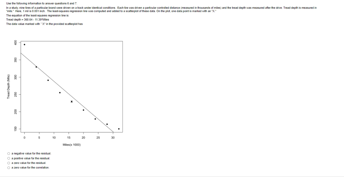
Use the following information to answer questions 6 and 7. In a study, nine tires of a particular brand were driven on a track under identical conditions. Each tire was driven a particular controlled distance (measured in thousands of miles) and the tread depth was measured after the drive. Tread depth is measured in "mils." Here, 1 mil is 0.001 inch. The least-squares regression line was computed and added to a scatterplot of these data. On the plot, one data point is marked with an "X" The equation of the least-squares regression line is: Tread depth = 360.64-11.39 Miles The data value marked with "X" in the provided scatterplot has Tread Depth (Mils) 00 350 ៖ 200 0 5 O a negative value for the residual. O a positive value for the residual. O a zero value for the residual O a zero value for the correlation. 10 15 Miles(x 1000) 20 25 30

A recent experiment included measuring the weight of a package of raw almonds.  This type of data would be considered a: Discrete variable or Continuous variable?

The datasetBody.xlsgives the percent of weight made up of body fat for 100 men as well as other variables such as Age, Weight (lb), Height (in), and circumference (cm) measurements for the Neck, Chest, Abdomen, Ankle, Biceps, and Wrist. We are interested in predicting body fat based on abdomen circumference. Find the equation of the regression line relating to body fat and abdomen circumference. Make a scatter-plot with a regression line. What body fat percent does the line predict for a person with an abdomen circumference of 110 cm? One of the men in the study had an abdomen circumference of 92.4 cm and a body fat of 22.5 percent. Find the residual that corresponds to this observation. Bodyfat Abdomen 32.3 115.6 22.5 92.4 22 86 12.3 85.2 20.5 95.6 22.6 100 28.7 103.1 21.3 89.6 29.9 110.3 21.3 100.5 29.9 100.5 20.4 98.9 16.9 90.3 14.7 83.3 10.8 73.7 26.7 94.9 11.3 86.7 18.1 87.5 8.8 82.8 11.8 83.3 11 83.6 14.9 87 31.9 108.5 17.3…

Listed below are the numbers of commuters and the number of parking spaces at different Metro-North railroad stations.      Use technology (calculator) to help you answer the following, and round to the 3 decimal places where rounding is necessary.                             .                                                      a. Find the linear regression line y = a + bx.    b. Are the variables positively or negatively related? c. Find and interpret r2.  Make sure to include what it means specific to this data set. d. Use your regression line to make a prediction for the number of parking spaces for a station with 900 e.  Identify and interpret the slope of the linear model.