
MATLAB: An Introduction with Applications
6th Edition
ISBN: 9781119256830
Author: Amos Gilat
Publisher: John Wiley & Sons Inc
expand_more
expand_more
format_list_bulleted
Related questions
Topic Video
Question
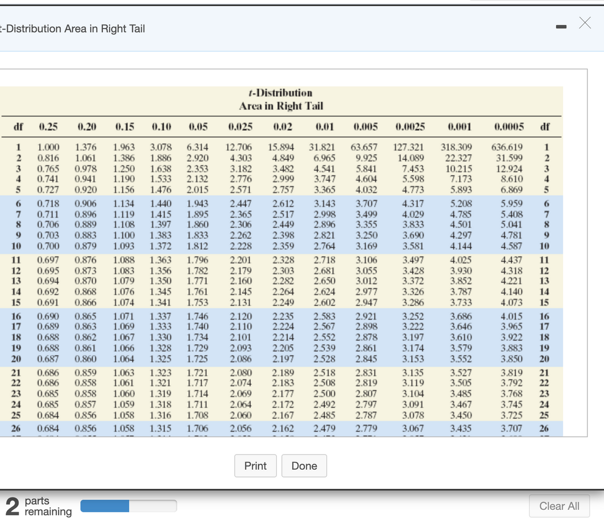
To test H0: μ=100 versus H1: μ≠100, a simple random
(a) If x=105 and s=9.1, compute the test statistic.
(b) If the researcher decides to test this hypothesis at the α=0.01 level of significance, determine the critical values. (Use a comma to separate answers as needed. Round to three decimal places as needed.)

Transcribed Image Text:t-Distribution Area in Right Tail
t-Distribution
Area in Right Tail
df
0.25
0.20
0.15
0.10
0.05
0.025
0.02
0.01
0.005
0.0025
0.001
0.0005
df
3.078
15.894
4.849
3.482
2.999
2.757
1.376
1.963
31.821
63.657
318.309
636.619
31.599
12.924
8.610
6.869
1
1.000
6.314
12.706
127.321
1
2.920
2.353
2.132
2.015
9.925
5.841
4.604
14.089
7.453
5.598
4.773
22.327
10.215
7.173
5.893
0.816
1.061
0.978
0.941
1.386
1.886
4.303
6.965
2
1.638
1.533
3
0.765
1.250
1.190
1.156
3.182
2.776
4.541
3.747
3
4
4
0.741
0.727
0.920
1.476
2.571
3.365
4.032
0.718
7
0.711
8
0.706
0.703
1.943
1.895
1.860
1.833
1.812
5.208
4.785
4.501
4.297
1.134
2.447
2.612
4.317
5.959
5.408
5.041
0.906
1.440
1.415
1.397
1.383
1.372
3.143
2.998
2.896
2.821
3.707
6.
0.896
0.889
0.883
1.119
1.108
1.100
1.093
2.517
2.449
2.398
2.359
3.499
3.355
3.250
3.169
4.029
3.833
3.690
3.581
2.365
2.306
7
8
2.262
2.228
4.781
4.587
9
10
0.700
0.879
2.764
4.144
10
0.876
0.873
0.870
1.088
1.363
1.796
1.782
1.771
1.761
1.753
3.106
3.055
3.012
3.497
3.428
3.372
4.025
3.930
3.852
3.787
3.733
11
4.437
0.697
0.695
0.694
0.692
2.201
2.179
2.160
2.328
2.718
11
12
13
1.083
1.079
1.356
1.350
2.303
2.282
2.264
2.681
2.650
2.624
2.602
4.318
4.221
12
13
2.145
2.131
2.977
2.947
14
0.868
1.076
1.345
3.326
3.286
4.140
14
15
0.691
0.866
1.074
1.341
2.249
4.073
15
3.686
3.646
3.610
3.579
3.552
16
17
0.690
0.689
0.688
0.688
0.687
0.865
0.863
0.862
1.071
1.069
1.067
1.337
1.333
1.330
1.328
1.746
1.740
2.120
2.110
2.235
2.224
2.214
2.205
2.583
2.567
2.921
2.898
2.878
3.252
3.222
4.015
3.965
3.922
16
17
1.734
1.729
18
2.101
2.552
3.197
18
3.883
3.850
19
0.861
1.066
2.093
2.539
2.861
3.174
19
20
0.860
1.064
1.325
1.725
2.086
2.197
2.528
2.845
3.153
20
0.686
0.686
0.685
0.685
0.859
0.858
0.858
21
22
1.063
1.061
1.323
1.321
1.319
1.721
1.717
2.080
2.074
2.189
2.183
2.177
2.172
2.167
2.518
2.508
3.527
3.505
3.485
2.831
2.819
3.135
3.119
3.819
3.792
3.768
3.745
3.725
21
22
1.060
1.059
1.058
2.069
2.064
2.060
2.500
2.492
2.485
2.807
2.797
2.787
23
1.714
3.104
23
0.857
0.856
3.091
3.078
3.467
3.450
24
1.318
1.711
24
25
0.684
1.316
1.708
25
26
0.684
0.856
1.058
1.315
1.706
2.056
2.162
2.479
2.779
3.067
3.435
3.707
26
Print
Done
parts
remaining
Clear All

Transcribed Image Text:t-Distribution Area in Right Tail
0.688
0.687
1.328
1.325
2.093
2.086
1.729
2.205
2.197
2.539
2.528
19
0.861
0.860
1.066
2.861
3.174
3.579
3.883
19
20
1.064
1.725
2.845
3.153
3.552
3.850
20
0.859
0.858
0.858
1.063
1.061
1.060
1.059
1.058
1.323
1.321
1.319
2.080
2.074
2.069
2.064
2.060
2.518
2.508
2.500
2.492
2.485
21
22
0.686
0.686
1.721
1.717
1.714
2.189
2.183
2.177
2.172
2.167
2.831
2.819
2.807
2.797
2.787
3.135
3.119
3.527
3.505
3.485
3.467
3.450
3.819
3.792
3.768
21
22
0.685
0.685
0.684
3.104
3.091
23
23
0.857
0.856
1.318
1.316
1.711
1.708
24
3.745
24
25
3.078
3.725
25
1.706
1.703
1.058
1.057
1.056
1.055
1.055
2.056
2.052
2.048
2.479
2.473
0.856
0.855
0.855
3.435
3.421
3.408
3.396
3.385
26
0.684
1.315
2.162
2.779
3.067
3.057
3.047
3.038
3.030
3.707
26
1.314
1.313
1.311
1.310
2.158
2.154
2.150
2.147
27
0.684
2.771
3.690
27
0.683
0.683
0.683
28
1.701
2.467
2.763
3.674
3.659
3.646
28
29
30
0.854
0.854
1.699
1.697
2.045
2.042
2.462
2.457
2.756
2.750
29
30
1.696
1.694
1.692
1.691
1.690
3.633
3.622
1.054
2.453
3.022
3.015
3.375
3.365
3.356
3.348
3.340
31
0.682
0.853
0.853
0.853
0.852
0.852
1.309
2.040
2.037
2.035
2.032
2.030
2.144
2.141
2.138
2.136
2.133
2.744
2.738
2.733
2.728
2.724
31
0.682
0.682
0.682
0.682
32
1.054
1.309
2.449
2.445
2.441
2.438
32
1.053
1.052
1.052
33
1.308
3.008
3.611
33
34
35
1.307
1.306
3.002
2.996
3.601
3.591
34
35
2.028
2.026
2.024
2.023
2.021
1.052
2.131
2.719
2.715
2.712
2.708
2.704
2.990
2.985
2.980
2.976
3.582
3.574
36
0.681
0.852
0.851
0.851
0.851
1.306
1.688
1.687
1.686
1.685
1.684
2.434
3.333
36
3.326
3.319
3.313
3.307
37
0.681
1.051 1.305
2.129 2.431
37
38
39
0.681
0.681
0.681
1.051
1.050
1.050
1.304
1.304
3.566
3.558
3.551
2.127
2.429
38
39
2.125 2.426
2.423
2.123
40
0.851
1.303
2.971
40
0.849
0.848
0.847
0.846
0.846
1.047 1.299
2.009
2.000
2.403
2.390
2.381
2.374
2.368
2.678
2.660
2.648
2.639
2.632
50
0.679
1.676
3.261
2.109
2.099
2.093
2.088
2.084
2.937
3.496
50
0.679
1.045 1.296
1.67
2.91.
3.460
3.23
3.211
3.195
60
60
0.678
0.678
0.677
3.435
3.416
3.402
70
1.044 1.294
1.043 1.292
1.042 1.291
1.667
1.664
1.662
1.994
1.990
2.899
2.887
2.878
70
80
80
90
1.987
3.183
90
100
1000
1.290
1.282
1.282
2.626
2.581
2.576
3.174
3.098
3.090
0.845
1.660
1.646
1.645
2.081
3.390
0.677
0.675
0.674
1.042
1.984
1.962
1.960
2.364
2.330
2.326
2.871
2.813
2.807
100
0.842
0.842
1.037
1.036
2.056
2.054
3.300 1000
3.291 z
df
0.25
0.20
0.15
0.10
0.05
0.025
0.02
0.01
0,005
0.0025
0.001
0.0005
df
Print
Done
parts
remaining
Clear All
Expert Solution
This question has been solved!
Explore an expertly crafted, step-by-step solution for a thorough understanding of key concepts.

This is a popular solution

Trending nowThis is a popular solution!

Step by stepSolved in 3 steps with 2 images

Knowledge Booster


Learn more about
Need a deep-dive on the concept behind this application? Look no further. Learn more about this topic, statistics and related others by exploring similar questions and additional content below.Similar questions
- A random sample of size 8 from a normal distribution has standard deviation s= 89. Test Ho:o=41 versus H, :0<41. Use the a=0.05 level of significance. Part 1 of 5 The hypotheses are provided above. This hypothesis test is a left-tailed test. Part: 1 /5 Part 2 of 5 Find the critical value. Critical value=arrow_forwardGive one method to increase statistical power and Which test statistic should you use if you are comparing two variances?arrow_forwardIf the researcher decides to test this hypothesis at the = 0.05 level of significance, determine the critical value. The critical value are=_ and=_. Round to three decimal places as needed.arrow_forward
- For the given data, (a) find the test statistic, (b) find the standardized test statistic, (c) decide whether the standardized test statistic is in the rejection region, and (d) decide whether you should reject or fail to reject the null hypothesis. The samples are random and independent. Claim: μ1<μ2, α=0.01.Sample statistics: x1=1220, n1=35, x2=1190, and n2=65. Population parameters: σ1=65 and σ2=105. Part 1 (a) The test statistic for μ1−μ2 is _____ b) The standardized test statistic for μ1−μ2 is _______ (Round to two decimal places as needed.) Part 3 (c) Is the standardized test statistic in the rejection region? Part 4 (d) Should you reject or fail to reject the null hypothesis? H0: μ1≥μ2; Ha: μ1<μ2. (Fail to reject/Reject) H0. At the % significance level, there is (not enough/ enough) evidence to support the claim.arrow_forwardUse the t-distribution and the given sample results to complete the test of the given hypotheses. Assume the results come from random samples, and if the sample sizes are small, assume the underlying distributions are relatively normal. Test Ho: M₁ = μ₂ vs Ha: ₁ ₂ using the sample results n₂ = = 80. Part 1 test statistic = i = (a) Give the test statistic and the p-value. Round your answer for the test statistic to two decimal places and your answer for the p-value to three decimal places. p-value = i 15.3, s₁ = 11.6 with n₁ = 100 and ₂ = 18.4, 82 = 14.3 witharrow_forwardWe want to use a z-test to determine if the sample mean is greater than 20 at the alpha = 0.05. What is the critical value(s)?arrow_forward
- Conduct a test at the α=0.01 level of significance by determining (a) the null and alternative hypotheses, (b) the test statistic, and (c) the P-value. Assume the samples were obtained independently from a large population using simple random sampling. Test whether p1>p2. The sample data are x1=124, n1=246, x2=136, and n2=311. (a) Choose the correct null and alternative hypotheses below. A. H0: p1=p2 versus H1: p1<p2 B. H0: p1=0 versus H1: p1≠0 C. H0: p1=p2 versus H1: p1>p2 D. H0: p1=p2 versus H1: p1≠p2 (b) Determine the test statistic. z0=nothing (Round to two decimal places as needed.) (c) Determine the P-value. The P-value is nothing. (Round to three decimal places as needed.) What is the result of this hypothesis test? A. Do not reject the null hypothesis because there is not sufficient evidence to conclude that p1<p2. B. Do not reject the null hypothesis because there is not…arrow_forwardConduct a test at the α=0.10 level of significance by determining Assume the samples were obtained independently from a large population using simple random sampling. Test whether p1>p2. The sample data are: x1=125, n1=259, x2=144, n2=311 (b) Determine the test statistic z0=?arrow_forwardUse the t-distribution and the sample results to complete the test of the hypotheses. Use a 5% significance level. Assume the results come from a random sample, and if the sample size is small, assume the underlying distribution is relatively normal.Test H0 : μ=15 vs Ha : μ>15 using the sample results x¯=17.2, s=6.4, with n=40. (a) Give the test statistic and the p-value.Round your answer for the test statistic to two decimal places and your answer for the p-value to three decimal places.test statistic = p-value =arrow_forward
- For the given data, (a) find the test statistic, (b) find the standardized test statistic, (c) decide whether the standardized test statistic is in the rejection region, and (d) decide whether you should reject or fail to reject the null hypothesis. The samples are random and independent. Claim: µ1 < H2, a = 0.01. Sample statistics: x, = 1215, n, = 45, x2 = 1195, and n2 = 75. Population statistics: 01 = 65 and 02 = 120. (a) The test statistic for H1 - H2 isarrow_forwardIndependent random samples, each containing 70 observations, were selected from two populations. Thearrow_forwardindependent random samples, each containing 90 observations, were selected from two populations. The samples from populations 1 and 2 produced 45 and 38 successes, respectively. Test;H0:(p1−p2)= 0 againstHa:(p1−p2)≠ 0Use α=0.03Test Statistic: P-Value:arrow_forward
arrow_back_ios
SEE MORE QUESTIONS
arrow_forward_ios
Recommended textbooks for you
- MATLAB: An Introduction with ApplicationsStatisticsISBN:9781119256830Author:Amos GilatPublisher:John Wiley & Sons Inc
 Probability and Statistics for Engineering and th...StatisticsISBN:9781305251809Author:Jay L. DevorePublisher:Cengage Learning
 Statistics for The Behavioral Sciences (MindTap C...StatisticsISBN:9781305504912Author:Frederick J Gravetter, Larry B. WallnauPublisher:Cengage Learning
  Elementary Statistics: Picturing the World (7th E...StatisticsISBN:9780134683416Author:Ron Larson, Betsy FarberPublisher:PEARSON
 The Basic Practice of StatisticsStatisticsISBN:9781319042578Author:David S. Moore, William I. Notz, Michael A. FlignerPublisher:W. H. Freeman
 Introduction to the Practice of StatisticsStatisticsISBN:9781319013387Author:David S. Moore, George P. McCabe, Bruce A. CraigPublisher:W. H. Freeman
MATLAB: An Introduction with Applications
Statistics
ISBN:9781119256830
Author:Amos Gilat
Publisher:John Wiley & Sons Inc
Probability and Statistics for Engineering and th...
Statistics
ISBN:9781305251809
Author:Jay L. Devore
Publisher:Cengage Learning
Statistics for The Behavioral Sciences (MindTap C...
Statistics
ISBN:9781305504912
Author:Frederick J Gravetter, Larry B. Wallnau
Publisher:Cengage Learning
Elementary Statistics: Picturing the World (7th E...
Statistics
ISBN:9780134683416
Author:Ron Larson, Betsy Farber
Publisher:PEARSON
The Basic Practice of Statistics
Statistics
ISBN:9781319042578
Author:David S. Moore, William I. Notz, Michael A. Fligner
Publisher:W. H. Freeman
Introduction to the Practice of Statistics
Statistics
ISBN:9781319013387
Author:David S. Moore, George P. McCabe, Bruce A. Craig
Publisher:W. H. Freeman