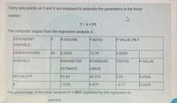
Thirty data points on Y and X are employed to estimate the parameters in the linear relation Y = a +bX. The computer output from the regression analysis is DEPENDENT VARIABLE: R-SQUARE F-RATIO P-VALUE ON F OBSERVATIONS: 30 0.5300 13.79 0.0009 VARIABLE PARAMETER STANDARD T-RATIO P-VALUE ESTIMATE ERROR INTERCEPT 93.54 46.210 2.02 0.0526 -3.25 0.875 -3.71 0.0009 The percentage of the total variation in Y NOT explained by the regression is

Suppose we estimated our multiple linear regression, all of the variables have p values below 0.05 (so they are statistically different from zero) but the intercept has p-value equal to p=0.343. What does it mean?

An analyst working for your firm provided an estimated log-linear demand function based on the natural logarithm of the quantity sold, price, and the average income of consumers. Results are summarized in the following table: SUMMARY OUTPUT Regression Statistics Multiple R R Square Adjusted R Square Standard Error Observations ANOVA Regression Residual Total Intercept LN Price LN Income df 0.968 0.937 0.933 0.003 30 SS MS F 2 0.003637484 0.001818742 202.48598 0.000242516 8.98206E-06 27 29 0.00388 Coefficients Standard Error 0.57 0.00 0.13 0.51 -0.08 0.15 t Stat 0.90 -19.50 1.13 P-value 0.37 0.00 0.27 Significance F 5.55598E-17 Lower 95% -0.65 -0.09 -0.12 How would a 4 percent increase in income impact the demand for your product? Demand would increase by 60 percent. Demand would increase by 0.6 percent. Demand would decrease by 60 percent. Demand would decrease by 0.6 percent. Upper 95% 1.68 -0.07 0.41

Please provide me with the correct answer, along with the calculations, and do not use any AI tools

QUESTION 10 Answer questions 10 to 16 based on the regression outputs given in Table 1& 2. Table 1 DATA4-1: Data on single family homes in University City community of San Diego, in 1990. price - sale price in thousands of dollars (Range 199. 9 505) sqft - square feet of living area (Range 1065 - 3000) Table 2 Model 1: OLS, using observations 1-14 Dependent variable: price coefficient std. error t-ratio p-value 52. 3509 0.138750 37. 2855 0.0187329 0. 1857 8. 20e-06 *** const sqft 7. 407 Me dependent var Sun squared resid R-squared F(1, 12) Log-likelihood Schwarz criterion 317. 4929 18273. 57 0. 820522 54. 86051 -70. 08421 145. 4465 Hannan-Quinn S.D. dependent var S.E. of regression Adjusted R-squared P-value (F) Akaike criterion 88. 49816 39. 02304 0. 805565 8. 20e-06 144. 1684 144. 0501 There are observations included in this dataset. It is a. data. O 12; cross-sectional 13; time-series data 14; cross-sectional In this regression model, sale price of a single-family house is the. the…

6) Suppose you have the following data on the price of orange and the quantity sold: Price per Pound (in Quantity Sold (in Dollars) Pounds) 0.50 0.75 1.00 1.25 1.50 10 7 699 5 2 Assume that the quantity sold (Y) is a linear function of the price (X), i.e. Y₁ =B₁ + B₂X₁ + ε₁ Estimate the population regression coefficients. (Do not use Computer)

q11-

The data for this question is given in the file 1.Q1.xlsx(see image)  and it refers to data for some cities X1 = total overall reported crime rate per 1 million residents X3 = annual police funding in $/resident X7 = % of people 25 years+ with at least 4 years of college   (a) Estimate a regression with X1 as the dependent variable and X3 and X7 as the independent variables. (b) Will additional education help to reduce total overall crime (lead to a statistically significant reduction in crime)? Please explain. (c) Will an increase in funding for the police departments help reduce total overall crime (lead to a statistically significant reduction in total overall crime)? Please explain. (d) If you were asked to recommend a policy to reduce crime, then, based only on the above regression results, would you choose to invest in education (local schools) or in additional funding for the police? Please explain.

The dependent variable in the regression in our cost driver analysis is which of the following? Company sales Total overhead cost for the entire period of time Total overhead cost per month

This exercise refers to the drunk driving panel data regression summarized below. Regression Analysis of the Effect of Drunk Driving Laws on Traffic Deaths Dependent variable: traffic fatility rate (deaths per 10,000). Regressor Beer tax Drinking age 18 Drinking age 19 Drinking age 20 Drinking age Mandatory jail or community service? Average vehicle miles per driver Unemployment rate Real income per capita (logarithm) Years State Effects? Time effects? (1) 0.41* (0.056) 1982-88 no no (2) (3) (4) -0.62** -0.76*** -0.42 (0.39) (0.33) (0.38) 0.023 (0.078) -0.014 (0.084) -0.023 -0.075 (0.053) (0.064) 0.034 -0.109*** (0.058) (0.058) no yes yes no yes Clustered standard errors? yes yes F-Statistics and p-Values Testing Exclusion of Groups of Variables Time effects=0 (5) -0.76** (0.36) 0.041 0.083 (0.111) (0.115) 0.006 0.015 (0.005) (0.011) -0.068* (0.016) 1.66* (0.66) 1982-88 1982-88 1982-88 1982-88 yes yes yes yes yes yes (6) -0.46 (0.39) -0.004 (0.022) 0.043 (0.101) 0.007 (0.005) -0.064*…