
MATLAB: An Introduction with Applications
6th Edition
ISBN: 9781119256830
Author: Amos Gilat
Publisher: John Wiley & Sons Inc
expand_more
expand_more
format_list_bulleted
Related questions
Concept explainers
Question
thumb_up100%
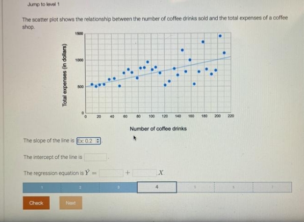

Transcribed Image Text:Jump to level 1
The scatter plot shows the relationship between the number of coffee drinks sold and the total expenses of a coffee
shop.
1500
1000
s00
20
40
60
80
100
120
140
160
180
200
220
Number of coffee drinks
The slope of the line is Ex 0.2 :
The intercept of the line is
The regression equation is Y
%3D
4.
Check
Next
Expert Solution
This question has been solved!
Explore an expertly crafted, step-by-step solution for a thorough understanding of key concepts.

This is a popular solution

Trending nowThis is a popular solution!

Step by stepSolved in 3 steps

Knowledge Booster


Learn more about
Need a deep-dive on the concept behind this application? Look no further. Learn more about this topic, statistics and related others by exploring similar questions and additional content below.Similar questions
- A set of X and Y scores has SSX = 15, SSY = 24, and SP = 60. The regression equation for these scores will have a slope constant of ______. a. 6 b. 5 c. 3 d. 4arrow_forwardAnnual high temperatures in a certain location have been tracked for several years. Let X represent the year and Y the high temperature. Assume that temperature is independent each year. Based on the data shown below, calculate the regression line (each value to two decimal places). First the slope and then the y-intercept. Y X 3 4 5 67 8 00 a 9 y 10.14 10.85 11.86 11.17 7.58 9.79 7.5 x+arrow_forwardPerform a linear regression analysis on the following data and determine the "a" coefficient (i.e., slope): Y 4.99 22.19 1.96 9.89 2.98 11 9 40.46 4.04 18.93 6.06 25 0.88 0.19 8.02 34.02 6.97 28.03arrow_forward
- Using the weights (Ib) and highway fuel consumption amounts (mi/gal) of the 48 cars listed in the accompanying data set, one gets this regression equation: y = 58 9-0.00749x, where x represents weight Complete parts (a) through (d). Click the icon to view the car data. 東 b. What are the specific values of the slope and y-intercept of the regression line? O A. The slope is 58.9 and the y-intercept is 0.007499. B. The slope is -0.00749 and the y-intercept is 58.9. O C. The slope is 58.9 and the y-intercept is -0.00749. O D. The slope is 0.00749 and the y-intercept is 58.9. c. What is the predictor variable? O A. The predictor variable is highway fuel consumption, which is represented by x. B. The predictor variable is weight, which is represented by x. O C. The predictor variable is weight, which is represented by y O D. The predictor variable is highway fuel consumption, which is represented by y. d. Assuming that there is a significant linear correlation between weight and highway fuel…arrow_forwardUse the data in the table below to complete parts (a) through (d). 39 33 40 47 42 50 59 56 51 24 22 27 32 30 31 31 27 29 Click the icon to view details on how to construct and interpret residual plots. (a) Find the equation of the regression line. (Round to three decimal places as needed.) (b) Construct a scatter plot of the data and draw the regression line. Plot the x-values on the horizontal axis and the y-values on the vertical axis. Choose the correct graph below. OA. В. Oc. OD. 34 70, (c) Construct a residual plot. Plot the x-values on the horizontal axis and the residuals on the vertical axis. Choose the correct graph below. O A. Ов. Oc. OD. (d) Determine if there are any patterns in the residual plot and explain what they suggest about the relationship between the variables. The residual plot a pattern because the residuals about 0. This implies the regression line a good representation of the relationship between the variables.arrow_forwardFind the equation of the regression line for the given data. Then construct a scatter plot of the data and draw the regression line. The table shows the shoe size and heights (in.) for 6 men. Shoe size, x Height, y Find the regression equation. ŷ=x+ (Round to three decimal places as needed.) Choose the correct graph below. O A. Height (in.) 75+ 65- 8 Shoe size N O B. Height (in.) 75+ 65+ 8.5 65.0 Shoe size 9.5 66.0 o 11.0 67.0 O C. Height (in.) 75 65 8 Shoe size 12.0 73.0 Q 13.0 71.0 D. Height (in.) 75- 65 13.5 73.0 Shoe size Q oarrow_forward
- Two variables are defined, a regression equation is given, and one data point is given. Study = number of hours spent studying for an exam Grade = grade on the exam GRADE= 41.0 + 3.7 (STUDY) THE DATA POINT IS A STUDENT WHO STUDIED 10 HOURS AND RECIEVED AN 81 ON THE EXAM…arrow_forwardn order for applicants to work for the foreign-service department, they must take a test in the language of the country where they plan to work. The data below shows the relationship between the number of years that applicants have studied a particular language and the grades they received on the proficiency exam. Find the equation of the regression line for the data. given Number of years, x 4 5 3 6 2 7 3 Grades on test, y 61 68 75 82 73 90 58 93 72 O A. y 6.910x+46.261 O B. -46.261x +6.910 O C. =6.910x-46.261 O D. = 46.261x-6.910 Next Time Remaining: 01:02:25 74°F Mostly 五 TTLarrow_forward
arrow_back_ios
arrow_forward_ios
Recommended textbooks for you
- MATLAB: An Introduction with ApplicationsStatisticsISBN:9781119256830Author:Amos GilatPublisher:John Wiley & Sons Inc
 Probability and Statistics for Engineering and th...StatisticsISBN:9781305251809Author:Jay L. DevorePublisher:Cengage Learning
 Statistics for The Behavioral Sciences (MindTap C...StatisticsISBN:9781305504912Author:Frederick J Gravetter, Larry B. WallnauPublisher:Cengage Learning
  Elementary Statistics: Picturing the World (7th E...StatisticsISBN:9780134683416Author:Ron Larson, Betsy FarberPublisher:PEARSON
 The Basic Practice of StatisticsStatisticsISBN:9781319042578Author:David S. Moore, William I. Notz, Michael A. FlignerPublisher:W. H. Freeman
 Introduction to the Practice of StatisticsStatisticsISBN:9781319013387Author:David S. Moore, George P. McCabe, Bruce A. CraigPublisher:W. H. Freeman
MATLAB: An Introduction with Applications
Statistics
ISBN:9781119256830
Author:Amos Gilat
Publisher:John Wiley & Sons Inc
Probability and Statistics for Engineering and th...
Statistics
ISBN:9781305251809
Author:Jay L. Devore
Publisher:Cengage Learning
Statistics for The Behavioral Sciences (MindTap C...
Statistics
ISBN:9781305504912
Author:Frederick J Gravetter, Larry B. Wallnau
Publisher:Cengage Learning
Elementary Statistics: Picturing the World (7th E...
Statistics
ISBN:9780134683416
Author:Ron Larson, Betsy Farber
Publisher:PEARSON
The Basic Practice of Statistics
Statistics
ISBN:9781319042578
Author:David S. Moore, William I. Notz, Michael A. Fligner
Publisher:W. H. Freeman
Introduction to the Practice of Statistics
Statistics
ISBN:9781319013387
Author:David S. Moore, George P. McCabe, Bruce A. Craig
Publisher:W. H. Freeman