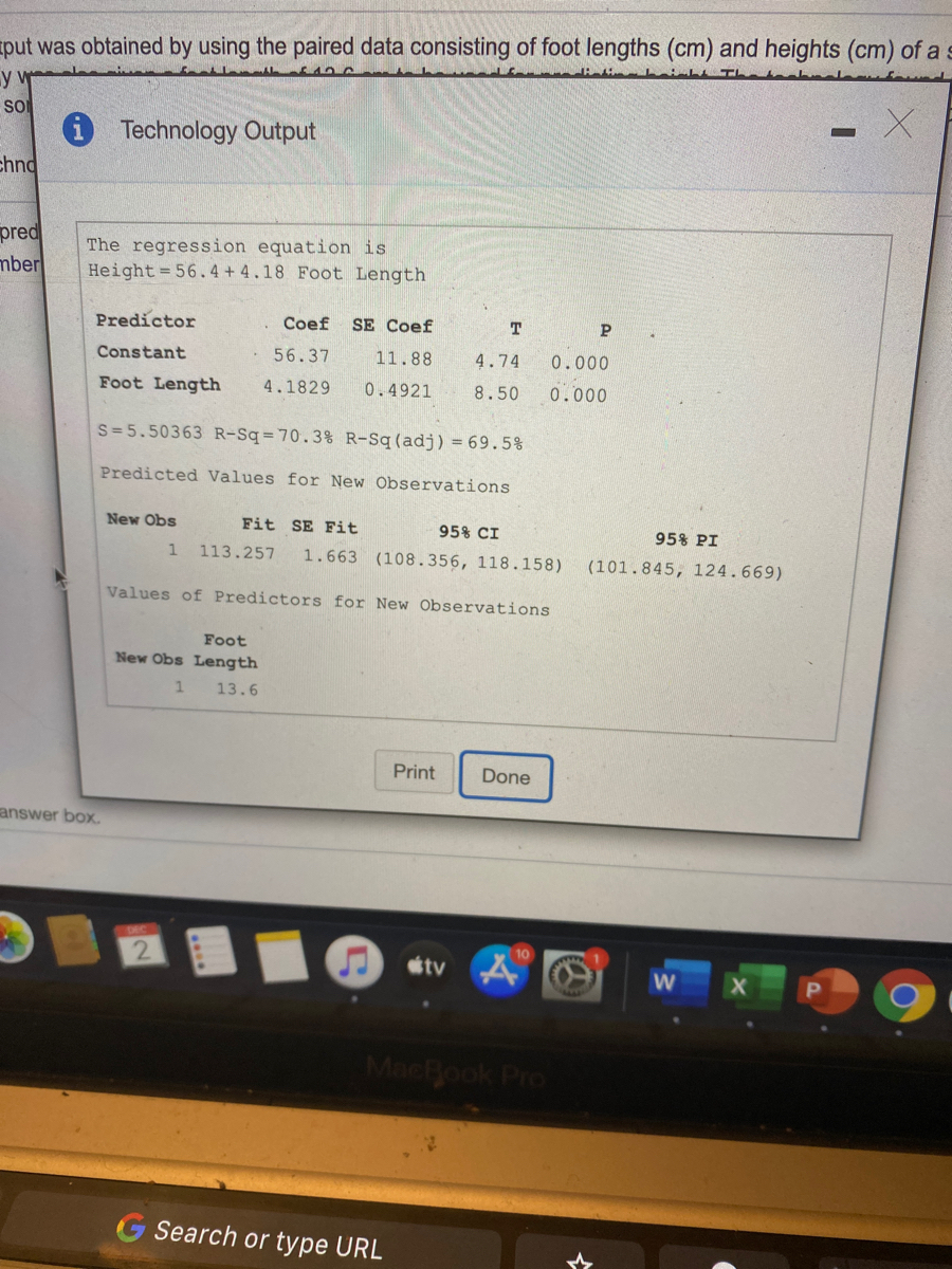
The regression equation is Height = 56.4+4.18 Foot Length %3D Predictor Coef SE Coef Constant 56.37 11.88 4.74 0.000 Foot Length 4.1829 0.4921 8.50 0.000 S=5.50363 R-Sq=70.3% R-Sq(adj) =69.5% Predicted Values for New Observations New Obs Fit SE Fit 95% CI 95% PI 1 113.257 1.663 (108.356, 118.158) (101.845 124 6601

A regression was run to determine if there is a relationship between hours of TV watched per day (x) and number of situps a person can do (y). The results of the regression were: y=ax+b a=-1.307 b=32.392 r²=0.675684 r=-0.822 Use this to predict the number of situps a person who watches 12.5 hours of TV can do (to one decimal place)

Exhibit 15-33 In a regression model involving 44 observations, the following estimated regression equation was obtained: y 10 - 4x12x2 + 8x3 + 8x4 For this model, SSR = 500 and SSE = 3500. Refer to Exhibit 15-33. The coefficient of determination for the above model is approximately -.875 .144 .125 .875

5:32 PM Tue Mar 1 + 94% A webassign.net A statistical program is recommended. A sales manager collected the following data on x=- years of experience and y = annual sales ($1,000s). The estimated regression equation for these data is ý = 83 + 4x. Years of Experience Annual Sales ($1,000s) Salesperson 1 80 3. 97 4 102 4 4. 107 6 103 6. 8 116 7 10 119 8 10 123 11 127 10 13 136 (a) Compute the residuals. Years of Annual Sales Experience ($1,000s) Residuals 80 87 3. 97 95 4 102 99 4 107 99 6. 103 107 8 116 115 10 119 123 10 123 123 11 127 127 13 136 135 Construct a residual plot. 16 16 12 12 8- 8 4 4 -4 -4 -8- -8- -12 -12 -16 -16 2 4 6 8 10 12 14 2. 4 6 8 10 12 14 Years of Experience Years of Exmerience Residuals Residuals

Given the following, determine the price of a Corolla that is six years old given the graph of the regression line.

You estimated a regression with the following output. Source | SS df MS Number of obs = 325 -------------+---------------------------------- F(1, 323) = 42850.36 Model | 285905003 1 285905003 Prob > F = 0.0000 Residual | 2155111.65 323 6672.17228 R-squared = 0.9925 -------------+---------------------------------- Adj R-squared = 0.9925 Total | 288060115 324 889074.429 Root MSE = 81.683 ------------------------------------------------------------------------------ Y | Coef. Std. Err. t P>|t| [95% Conf. Interval] -------------+---------------------------------------------------------------- X | 11.83842 .0571895 207.00 0.000 11.72591 11.95093 _cons | 52.14457 5.949458 8.76 0.000 40.43999 63.84915…

Please fill in the blanks and select the correct answers over the image provided. Thank you

You estimated a regression with the following output.         Source |       SS           df       MS      Number of obs   =       246 -------------+----------------------------------   F(1, 244)       =  16642.70        Model |   187647307         1   187647307   Prob > F        =    0.0000     Residual |  2751112.55       244  11275.0514   R-squared       =    0.9856 -------------+----------------------------------   Adj R-squared   =    0.9855        Total |   190398419       245  777136.405   Root MSE        =    106.18   ------------------------------------------------------------------------------            Y |      Coef.   Std. Err.      t    P>|t|     [95% Conf. Interval] -------------+----------------------------------------------------------------            X |   13.79687    .106947   129.01   0.000     13.58621    14.00753        _cons |   17.60822   9.208341     1.91   0.057    -.5297613     35.7462…

From the results shown above, write the regression equation.

You estimated a regression with the following output.         Source |       SS           df       MS      Number of obs   =       423 -------------+----------------------------------   F(1, 421)       =    267.80        Model |  8758968.84         1  8758968.84   Prob > F        =    0.0000     Residual |  13769523.8       421  32706.7074   R-squared       =    0.3888 -------------+----------------------------------   Adj R-squared   =    0.3873        Total |  22528492.7       422  53385.0537   Root MSE        =    180.85   ------------------------------------------------------------------------------            Y |      Coef.   Std. Err.      t    P>|t|     [95% Conf. Interval] -------------+----------------------------------------------------------------            X |   6.150402   .3758334    16.36   0.000     5.411658    6.889145        _cons |  -8.022201   24.02003    -0.33   0.739    -55.23632    39.19192…