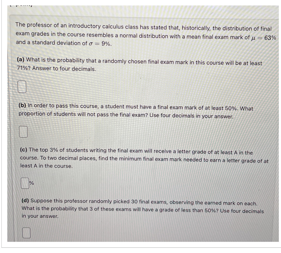
The professor of an introductory calculus class has stated that, historically, the distribution of final exam grades in the course resembles a normal distribution with a mean final exam mark of = 63% and a standard deviation of σ = 9%. (a) What is the probability that a randomly chosen final exam mark in this course will be at least 71%? Answer to four decimals. (b) In order to pass this course, a student must have a final exam mark of at least 50%. What proportion of students will not pass the final exam? Use four decimals in your answer. (c) The top 3% of students writing the final exam will receive a letter grade of at least A in the course. To two decimal places, find the minimum final exam mark needed to earn a letter grade of at least A in the course. % (d) Suppose this professor randomly picked 30 final exams, observing the earned mark on each. What is the probability that 3 of these exams will have a grade of less than 50%? Use four decimals in your answer.

You now have 10,000, all of which is invested in a sports team. Each year there is a 60% chance that the value of the team will increase by 60% and a 40% chance that the value of the team will decrease by 60%. Estimate the mean and median value of your investment after 50 years. Explain the large difference between the estimated mean and median.

Based on Marcus (1990). The Balboa mutual fund has beaten the Standard and Poors 500 during 11 of the last 13 years. People use this as an argument that you can beat the market. Here is another way to look at it that shows that Balboas beating the market 11 out of 13 times is not unusual. Consider 50 mutual funds, each of which has a 50% chance of beating the market during a given year. Use simulation to estimate the probability that over a 13-year period the best of the 50 mutual funds will beat the market for at least 11 out of 13 years. This probability turns out to exceed 40%, which means that the best mutual fund beating the market 11 out of 13 years is not an unusual occurrence after all.

Based on Babich (1992). Suppose that each week each of 300 families buys a gallon of orange juice from company A, B, or C. Let pA denote the probability that a gallon produced by company A is of unsatisfactory quality, and define pB and pC similarly for companies B and C. If the last gallon of juice purchased by a family is satisfactory, the next week they will purchase a gallon of juice from the same company. If the last gallon of juice purchased by a family is not satisfactory, the family will purchase a gallon from a competitor. Consider a week in which A families have purchased juice A, B families have purchased juice B, and C families have purchased juice C. Assume that families that switch brands during a period are allocated to the remaining brands in a manner that is proportional to the current market shares of the other brands. For example, if a customer switches from brand A, there is probability B/(B + C) that he will switch to brand B and probability C/(B + C) that he will switch to brand C. Suppose that the market is currently divided equally: 10,000 families for each of the three brands. a. After a year, what will the market share for each firm be? Assume pA = 0.10, pB = 0.15, and pC = 0.20. (Hint: You will need to use the RISKBINOMLAL function to see how many people switch from A and then use the RISKBENOMIAL function again to see how many switch from A to B and from A to C. However, if your model requires more RISKBINOMIAL functions than the number allowed in the academic version of @RISK, remember that you can instead use the BENOM.INV (or the old CRITBENOM) function to generate binomially distributed random numbers. This takes the form =BINOM.INV (ntrials, psuccess, RAND()).) b. Suppose a 1% increase in market share is worth 10,000 per week to company A. Company A believes that for a cost of 1 million per year it can cut the percentage of unsatisfactory juice cartons in half. Is this worthwhile? (Use the same values of pA, pB, and pC as in part a.)

A new edition of a very popular textbook will be published a year from now. The publisher currently has 1000 copies on hand and is deciding whether to do another printing before the new edition comes out. The publisher estimates that demand for the book during the next year is governed by the probability distribution in the file P10_31.xlsx. A production run incurs a fixed cost of 15,000 plus a variable cost of 20 per book printed. Books are sold for 190 per book. Any demand that cannot be met incurs a penalty cost of 30 per book, due to loss of goodwill. Up to 1000 of any leftover books can be sold to Barnes and Noble for 45 per book. The publisher is interested in maximizing expected profit. The following print-run sizes are under consideration: 0 (no production run) to 16,000 in increments of 2000. What decision would you recommend? Use simulation with 1000 replications. For your optimal decision, the publisher can be 90% certain that the actual profit associated with remaining sales of the current edition will be between what two values?

You have 5 and your opponent has 10. You flip a fair coin and if heads comes up, your opponent pays you 1. If tails comes up, you pay your opponent 1. The game is finished when one player has all the money or after 100 tosses, whichever comes first. Use simulation to estimate the probability that you end up with all the money and the probability that neither of you goes broke in 100 tosses.

Play Things is developing a new Lady Gaga doll. The company has made the following assumptions: The doll will sell for a random number of years from 1 to 10. Each of these 10 possibilities is equally likely. At the beginning of year 1, the potential market for the doll is two million. The potential market grows by an average of 4% per year. The company is 95% sure that the growth in the potential market during any year will be between 2.5% and 5.5%. It uses a normal distribution to model this. The company believes its share of the potential market during year 1 will be at worst 30%, most likely 50%, and at best 60%. It uses a triangular distribution to model this. The variable cost of producing a doll during year 1 has a triangular distribution with parameters 15, 17, and 20. The current selling price is 45. Each year, the variable cost of producing the doll will increase by an amount that is triangularly distributed with parameters 2.5%, 3%, and 3.5%. You can assume that once this change is generated, it will be the same for each year. You can also assume that the company will change its selling price by the same percentage each year. The fixed cost of developing the doll (which is incurred right away, at time 0) has a triangular distribution with parameters 5 million, 7.5 million, and 12 million. Right now there is one competitor in the market. During each year that begins with four or fewer competitors, there is a 25% chance that a new competitor will enter the market. Year t sales (for t 1) are determined as follows. Suppose that at the end of year t 1, n competitors are present (including Play Things). Then during year t, a fraction 0.9 0.1n of the company's loyal customers (last year's purchasers) will buy a doll from Play Things this year, and a fraction 0.2 0.04n of customers currently in the market ho did not purchase a doll last year will purchase a doll from Play Things this year. Adding these two provides the mean sales for this year. Then the actual sales this year is normally distributed with this mean and standard deviation equal to 7.5% of the mean. a. Use @RISK to estimate the expected NPV of this project. b. Use the percentiles in @ RISKs output to find an interval such that you are 95% certain that the companys actual NPV will be within this interval.

You now have 5000. You will toss a fair coin four times. Before each toss you can bet any amount of your money (including none) on the outcome of the toss. If heads comes up, you win the amount you bet. If tails comes up, you lose the amount you bet. Your goal is to reach 15,000. It turns out that you can maximize your chance of reaching 15,000 by betting either the money you have on hand or 15,000 minus the money you have on hand, whichever is smaller. Use simulation to estimate the probability that you will reach your goal with this betting strategy.

Software development is an inherently risky and uncertain process. For example, there are many examples of software that couldnt be finished by the scheduled release datebugs still remained and features werent ready. (Many people believe this was the case with Office 2007.) How might you simulate the development of a software product? What random inputs would be required? Which outputs would be of interest? Which measures of the probability distributions of these outputs would be most important?

Assume that all of a companys job applicants must take a test, and that the scores on this test are normally distributed. The selection ratio is the cutoff point used by the company in its hiring process. For example, a selection ratio of 25% means that the company will accept applicants for jobs who rank in the top 25% of all applicants. If the company chooses a selection ratio of 25%, the average test score of those selected will be 1.27 standard deviations above average. Use simulation to verify this fact, proceeding as follows. a. Show that if the company wants to accept only the top 25% of all applicants, it should accept applicants whose test scores are at least 0.674 standard deviation above average. (No simulation is required here. Just use the appropriate Excel normal function.) b. Now generate 1000 test scores from a normal distribution with mean 0 and standard deviation 1. The average test score of those selected is the average of the scores that are at least 0.674. To determine this, use Excels DAVERAGE function. To do so, put the heading Score in cell A3, generate the 1000 test scores in the range A4:A1003, and name the range A3:A1003 Data. In cells C3 and C4, enter the labels Score and 0.674. (The range C3:C4 is called the criterion range.) Then calculate the average of all applicants who will be hired by entering the formula =DAVERAGE(Data, "Score", C3:C4) in any cell. This average should be close to the theoretical average, 1.27. This formula works as follows. Excel finds all observations in the Data range that satisfy the criterion described in the range C3:C4 (Score0.674). Then it averages the values in the Score column (the second argument of DAVERAGE) corresponding to these entries. See online help for more about Excels database D functions. c. What information would the company need to determine an optimal selection ratio? How could it determine the optimal selection ratio?