
Related questions
Concept explainers
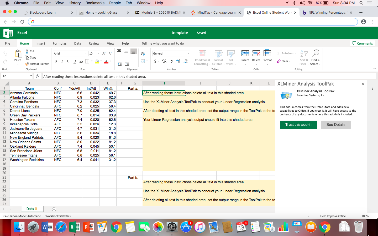
The National Football League (NFL) records a variety of performance data for individuals and teams. To investigate the importance of passing on the percentage of games won by a team, the data in the Excel Online file below show the conference (Conf), average number of passing yards per attempt (Yds/Att), the number of interceptions thrown per attempt (Int/Att), and the percentage of games won (Win%) for a random sample of 16 NFL teams for a season. Construct a spreadsheet to answer the following questions.
-
Develop the estimated regression equation that could be used to predict the percentage of games won given the average number of passing yards per attempt (to 1 decimal).
-
Develop the estimated regression equation that could be used to predict the percentage of games won given the number of interceptions thrown per attempt (to 1 decimal).
-
Develop the estimated regression equation that could be used to predict the percentage of games won given the average number of passing yards per attempt and the number of interceptions thrown per attempt (to 1 decimal).
-
The average number of passing yards per attempt for the Kansas City Chiefs was 6.2 and the number of interceptions thrown per attempt was 0.036. Use the estimated regression equation developed in part (c) to predict the percentage of games won by the Kansas City Chiefs. (Note: For this season the Kansas City Chiefs' record was 7 wins and 9 losses.) Compare your prediction to the actual percentage of games won by the Kansas City Chiefs (to whole number).
Predicted percentage Actual percentage _____<>=


Trending nowThis is a popular solution!

Step by stepSolved in 4 steps with 4 images


- In Exercises 33 to 36, determine whether or not the conditions for using two-sample t procedures are met. 33. Shoes How many pairs of shoes do teenagers have? To find out, a group of AP® Statistics students conducted a survey. They selected a random sample of 20 female students and a separate random sample Females 333 95 4332 66 410 8 9 100 7 0 0 4455 WW~~ 1 1 2 2 2 Males 4 3 555677778 0000124 3 58 Key: 22 represents a male student with 22 pairs of shoes.arrow_forwardDO THIS TYPEWRITTEN FOR UPVOTEarrow_forwardA statistical program is recommended. The Condé Nast Traveler Gold List provides ratings for the top 20 small cruise ships. The data shown below are the scores each ship received based upon the results from Condé Nast Traveler's Annual Readers' Choice Survey. Each score represents the percentage of respondents who rated a ship as excellent or very good on several criteria, including Shore Excursions and Food/Dining. An overall score was also reported and used to rank the ships. The highest ranked ship, the Seabourn Odyssey, has an overall score of 94.4, the highest component of which is 97.8 for Food/Dining. Shore Ship Overall Food/Dining Excursions Seabourn Odyssey 94.4 90.9 97.8 Seabourn Pride 93.0 84.2 96.7 National Geographic Endeavor 92.9 100.0 88.5 Seabourn Sojourn 91.3 94.8 97.1 Paul Gauguin 90.5 87.9 91.2 Seabourn Legend 90.3 82.1 98.8 Seabourn Spirit 90.2 86.3 92.0 Silver Explorer 89.9 92.6 88.9 Silver Spirit 89.4 85.9 90.8 Seven Seas Navigator 89.2 83.3 90.5 Silver Whisperer…arrow_forward
- Each year forbes ranks the world’s most valuable brands. A portion of the data for 82 ofthe brands in the 2013 forbes list is shown in Table 2.12 (forbes website, february, 2014).The data set includes the following variables:brand: The name of the brand.Industry: The type of industry associated with the brand, labeled Automotive& Luxury, Consumer Packaged Goods, financial Services, Other, Technology.brand Value ($ billions): A measure of the brand’s value in billions of dollarsdeveloped by forbes based on a variety of financial information about the brand.1-Yr Value Change (%): The percentage change in the value of the brand over theprevious year.brand Revenue ($ billions): The total revenue in billions of dollars for the brand.a. Prepare a crosstabulation of the data on Industry (rows) and brand Value ($ billions).Use classes of 0–10, 10–20, 20–30, 30–40, 40–50, and 50–60 for brand Value($ billions).b. Prepare a frequency distribution for the data on Industry.arrow_forwardA marketing firm is doing research for an internet-based company. It wants to appeal to the age group of people who spend the most money online. The company wants to know if there is a difference in the mean amount of money people spend per morith on Internet purchases depending on their age bracket. The marketing firm looked at two age groups, 18-24 years and 25-30 years, and collected the data shown in the following table. Let Population 1 be the amount of money spent per month on internet purchases by people in the 18-24 age bracket and Population 2 be the amount of money spent per month on internet purchases by people in the 25-30 age bracket. Assume that the population variances are not the same. Internet Spending per Month 18-24 Years Answer Mean Amount Spent Standard Deviation Sample Size Step 1 of 2: Construct a 99 % confidence interval for the true difference between the mean amounts of money per month that people in these two age groups spend on Internet purchases. Round the…arrow_forwardIn marketing children’s products, it is extremely important to produce television commercials that hold the attention of the children who view them. A psychologist hired by a marketing research firm wants to determine whether differences in attention span exist among advertisements for different types of products. A number of children under 10 years of age are asked to watch one 60-second commercial for one of three types of products, and their attention spans are measured in seconds. The results are shown in the accompanying table: Type of Product Advertised Toys/Games Food/Candy Children’s Clothing 42 55 30 45 58 35 48 52 42 40 60 32 50 57 38 b). What type of error is possible and describe this error in terms of the problem.arrow_forward
- What is the proportion of the blood type O?arrow_forwardA randomly sampled group of patients at a major U.S. regional hospital became part of a nutrition study on dietary habits. Part of the study consisted of a 50-question survey asking about types of foods consumed. Each question was scored on a scale from one (most unhealthy behavior) to five (most healthy behavior). The answers were summed and averaged. The population of interest is the patients at the regional hospital. A prior survey of patients had found the mean score for the population of patients to be μ=2.9 After careful review of these data, the hospital nutritionist decided that patients could benefit from nutrition education. The current survey was implemented after patients were subjected to this education, and it produced the following sample statistics for the 15 patients sampled: x¯=3.5 and s=1.2 We would like to know if the education improved nutrition behavior. We test the hypotheses H0:μ=2.9 versus Ha:μ>2.9. The tt test to be used has the test statistic: Answer:arrow_forwardA contributor for the local newspaper is writing an article for the weekly fitness section. To prepare for the story, she conducts a study to compare the exercise habits of people who exercise in the morning to the exercise habits of people who work out in the afternoon or evening. She selects three different health centers from which to draw her samples. The 57 people she sampled who work out in the morning have a mean of 4.8 hours of exercise each week. The 56 people surveyed who exercise in the afternoon or evening have a mean of 4.2 hours of exercise each week. Assume that the weekly exercise times have a population standard deviation of 0.8 hours for people who exercise in the morning and 0.3 hours for people who exercise in the afternoon or evening. Let Population 1 be people who exercise in the morning and Population 2 be people who exercise in the afternoon or evening. Step 1 of 2 : Construct a 95% confidence interval for the true difference between the mean amounts…arrow_forward
- The home run percentage is the number of home runs per 100 times at bat. A random sample of 43 professional baseball players gave the following data for home run percentages.arrow_forwardfill blanks underlines.arrow_forwardA County Board of Supervisors has appointed an urban planning committee to evaluate proposed community development projects. The committee is analyzing, among other things, data on household incomes in two cities within the county. They have collected data on the income of 77 households in each of the two cities. The histograms below show the distributions of the two sets of incomes (in thousands of dollars). Each histogram shows household income on the horizontal axis and number of households on the vertical axis. The means and standard deviations for the data sets are also given. City A City B 25+ 20+ 15+ 10+ 5- ← 10 20 30 40 50 60 70 80 90 100 City A mean: 73.96 thousand dollars City A standard deviation: 20.30 thousand dollars Explanation 25- 20- 15- 104 5+ 10 (a) Identify the data set for which it is appropriate to use the Empirical Rule. It is appropriate to use the Empirical Rule for the (Choose one) ▼ data set. 20 30 The committee wants to use the Empirical Rule to make some…arrow_forward
- MATLAB: An Introduction with ApplicationsStatisticsISBN:9781119256830Author:Amos GilatPublisher:John Wiley & Sons Inc
 Probability and Statistics for Engineering and th...StatisticsISBN:9781305251809Author:Jay L. DevorePublisher:Cengage Learning
 Statistics for The Behavioral Sciences (MindTap C...StatisticsISBN:9781305504912Author:Frederick J Gravetter, Larry B. WallnauPublisher:Cengage Learning
  Elementary Statistics: Picturing the World (7th E...StatisticsISBN:9780134683416Author:Ron Larson, Betsy FarberPublisher:PEARSON
 The Basic Practice of StatisticsStatisticsISBN:9781319042578Author:David S. Moore, William I. Notz, Michael A. FlignerPublisher:W. H. Freeman
 Introduction to the Practice of StatisticsStatisticsISBN:9781319013387Author:David S. Moore, George P. McCabe, Bruce A. CraigPublisher:W. H. Freeman