
MATLAB: An Introduction with Applications
6th Edition
ISBN: 9781119256830
Author: Amos Gilat
Publisher: John Wiley & Sons Inc
expand_more
expand_more
format_list_bulleted
Related questions
Concept explainers
Topic Video
Question
thumb_up100%
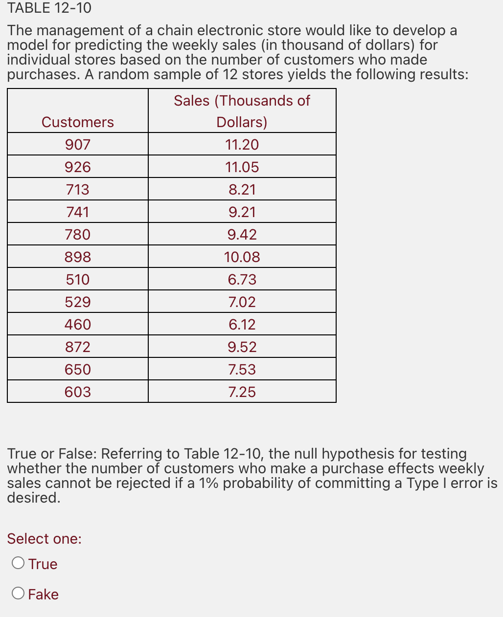

Transcribed Image Text:TABLE 12-10
The management of a chain electronic store would like to develop a
model for predicting the weekly sales (in thousand of dollars) for
individual stores based on the number of customers who made
purchases. A random sample of 12 stores yields the following results:
Sales (Thousands of
Customers
Dollars)
907
11.20
926
11.05
713
8.21
741
9.21
780
9.42
898
10.08
510
6.73
529
7.02
460
6.12
872
9.52
650
7.53
603
7.25
True or False: Referring to Table 12-10, the nulI hypothesis for testing
whether the number of customers who make a purchase effects weekly
sales cannot be rejected if a 1% probability of committing a Type I error is
desired.
Select one:
O True
O Fake
Expert Solution
This question has been solved!
Explore an expertly crafted, step-by-step solution for a thorough understanding of key concepts.

This is a popular solution

Trending nowThis is a popular solution!

Step by stepSolved in 2 steps

Knowledge Booster


Learn more about
Need a deep-dive on the concept behind this application? Look no further. Learn more about this topic, statistics and related others by exploring similar questions and additional content below.Similar questions
- A government agency computed the proportion of U.S. residents who lived in each of four geographic regions in a particular year. Then a simple random sample was drawn of 1000 people living in the United States in the current year. The following table presents the results. Region Past YearProportion ObservedCounts Northeast 0.171 150 Midwest 0.245 235 South 0.357 398 West 0.227 217 Send data to Excel Can you conclude that the proportions of people living in the various regions changed between the current year and the past year? Use the 0.05 level of significance and the P-value method with the TI-84 Plus calculator. What the P value?arrow_forwardAn article about the California lottery gave the following information on the age distribution of adults in California: 35% are between 18 and 34 years old, 51% are between 35 and 64 years old, and 14% are 65 years old or older. The article also gave information on the age distribution of those who purchase lottery tickets. The following table is consistent with the values given in the article. Suppose that the data resulted from a random sample of 200 lottery ticket purchasers. Based on these sample data, is it reasonable to conclude that one or more of these three age groups buys a disproportionate share of lottery tickets? Use a chi-square goodness-of-fit test with ? = 0.05. Age of Purchaser Frequency 18–34 36 35–64 130 65 and over 34 Calculate the test statistic. (Round your answer to two decimal places.) ?2 = Use technology to calculate the P-value. (Round your answer to four decimal places.) P-value = What can you conclude? The data strong evidence to conclude…arrow_forwardThe owner of Maumee Ford-Volvo wants to study the relationship between the age of a car and its selling price. Listed below is a random sample of 12 used cars sold at the dealership during the last year. Car Age (years) Selling Price ($000) 1 11 12.1 2 8 10.5 3 14 5.7 4 17 4.9 5 9 5.0 6 8 13.4 7 10 10.5 8 14 9.0 9 13 9.0 10 17 4.5 11 6 12.5 12 6 11.5 Click here for the Excel Data Filea. Determine the regression equation. (Negative amounts should be indicated by a minus sign. Round your answers to 3 decimal places.) a= b= Estimate the selling price of an 7-year-old car (in $000). (Round your answer to 3 decimal places.) Interpret the regression equation (in dollars). (Round your answer to the nearest dollar amount.)arrow_forward
- The price of a share of stock divided by the company's estimated future earnings per share is called the P/E ratio. High P/E ratios usually indicate "growth" stocks, or maybe stocks that are simply overpriced. Low P/E ratios indicate "value" stocks or bargain stocks. A random sample of 51 of the largest companies in the United States gave the following P/E ratiost. 9 20 11 35 19 13 15 21 29 53 16 26 21 14 21 27 10 12 47 14 40 18 60 72 33 14 8 49 5 16 8 19 12 31 67 51 26 18 17 20 19 13 25 23 27 44 20 27 19 18 32 (a) Use a calculator with mean and sample standard deviation keys to find the sample mean x and sample standard deviation s. (Round your answers to one decimal place.) (b) Find a 90% confidence interval for the P/E population mean u of all large U.S. companies. (Round your answers to one decimal place.) lower limit upper limit (c) Find a 99% confidence interval for the P/E population mean u of all large U.S. companies. (Round your answers to one decimal place.) lower limit upper…arrow_forwardIs there a relation between incidents of child abuse and number of runaway children? A random sample of cities (over 10,000 population) gave the following information about the number of reported incidents of child abuse and the number of runaway children. (Reference: Federal Bureau of Investigation, U.S. Department of Justice.) City 1 2 3 4 5 6 7 8 9 10 11 12 13 14 15 Abuse cases 113 33 41 60 52 99 31 56 15 67 106 59 45 74 84 Runaways 648 188 285 687 421 590 284 277 162 473 600 432 317 580 592 Use a 1% level of significance to test the claim that there is a monotone-increasing relationship between the ranks of incidents of abuse and number of runaway children. (a) Rank-order abuse using 1 as the largest data value. Also rank-order runaways using 1 as the largest data value. Then construct a table of ranks to be used for a Spearman rank correlation test. City Abuse CasesRank x RunawaysRank y d = x - y d2 123456789101112131415 Σd2 = (b) What is the level of…arrow_forwardLast school year, the student body of a local university consisted of 35% freshmen, 24% sophomores, 26% juniors, and 15% seniors. A sample of 300 students taken from this year's student body showed the following number of students in each classification. Freshmen 90 Sophomores 60 Juniors 90 Seniors 60 We are interested in determining whether or not there has been a significant change in the classifications between the last school year and this school year. The calculated value for the test statistic equals a. 0.5444 b. 2.789 c. 10.989 d. 15.231arrow_forward
- The mean birthweight of an infant is thought to be associated with the smoking status of the mother during the first trimester of the pregnancy. Consider the following data from mothers divided into four categories according to smoking habits, and the corresponding birthweights of their children. Group 1: Mother is a non smoker (NON): 7.5, 6.2, 6.9, 7.4, 9.2, 8.3, 7.6 Group 2: Mother is an ex-smoker (EX): 5.8, 7.3, 8.2, 7.1, 7.8 Group 3: Mother is a current smoker, smokes less than 1 pack per day (CUR < 1) 5.9, 6.2, 5.8, 4.7, 8.3, 7.2, 6.2 Group 4: Mother is a current smoker, smokes more than or equal to 1 pack per day (Cur ≥ 1) 6.2, 6.8, 5.7, 4.9, 6.2, 7.1, 5.8, 5.4 Using Stata test whether or not the mean birthweights are equal across all four groups at the alpha = 0.05 level. What are your null and alternative hypothesis? Ο HO: μ_1== μ_2 HA: μ_1=\= μ_2 O HO: μ_i== u_j for all i and j HA: μ_i=\= μ_j for all i and j O HO: μ_i == μ_j for all i and j HA: μ_i=\= μ_j for at least one i,j…arrow_forwardHow do the average weekly incomes of electricians and carpenters compare? A random sample of 17 regions in the United States gave the following information about average weekly income (in dollars). (Reference: U.S. Department of Labor, Bureau of Labor Statistics.) Region 1 2 3 4 5 6 7 8 9 Electricians 464 715 597 464 736 694 744 571 806 Carpenters 542 813 513 476 688 503 789 653 474 Region 10 11 12 13 14 15 16 17 Electricians 592 594 702 579 868 598 597 654 Carpenters 489 647 676 384 817 605 556 505 Does this information indicate a difference (either way) in the average weekly incomes of electricians compared to those of carpenters? Use a 5% level of significance. (a) What is the level of significance? (b) Compute the sample test statistic. (c) Find the P-value of the sample test statistic.arrow_forwardUsed car auctions give car dealers an opportunity to increase their used car inventory by purchasing cars used as rental cars, assigned to company executives, and other similar activities. Suppose population 1 is all black cars sold at used car auctions, and population 2 is all white cars sold at used car auctions. Of interest is to estimate the difference in the mean sale price of all black cars sold at used car auctions and the mean sale price of all white cars sold at used car auctions. Based on this, using both the appropriate symbol and in words, state the one parameter of interest.arrow_forward
- Pavanarrow_forwardHospitals In a study of births in New York State, data were collected from four hospitals coded as follows: (1) Albany Medical Center; (1438) Bellevue Hospital Center; (66) Olean General Hospital; (413) Strong Memorial Hospital. Does it make sense to calculate the average (mean) of the numbers 1, 1438, 66, and 413?arrow_forward
arrow_back_ios
arrow_forward_ios
Recommended textbooks for you
- MATLAB: An Introduction with ApplicationsStatisticsISBN:9781119256830Author:Amos GilatPublisher:John Wiley & Sons Inc
 Probability and Statistics for Engineering and th...StatisticsISBN:9781305251809Author:Jay L. DevorePublisher:Cengage Learning
 Statistics for The Behavioral Sciences (MindTap C...StatisticsISBN:9781305504912Author:Frederick J Gravetter, Larry B. WallnauPublisher:Cengage Learning
  Elementary Statistics: Picturing the World (7th E...StatisticsISBN:9780134683416Author:Ron Larson, Betsy FarberPublisher:PEARSON
 The Basic Practice of StatisticsStatisticsISBN:9781319042578Author:David S. Moore, William I. Notz, Michael A. FlignerPublisher:W. H. Freeman
 Introduction to the Practice of StatisticsStatisticsISBN:9781319013387Author:David S. Moore, George P. McCabe, Bruce A. CraigPublisher:W. H. Freeman
MATLAB: An Introduction with Applications
Statistics
ISBN:9781119256830
Author:Amos Gilat
Publisher:John Wiley & Sons Inc
Probability and Statistics for Engineering and th...
Statistics
ISBN:9781305251809
Author:Jay L. Devore
Publisher:Cengage Learning
Statistics for The Behavioral Sciences (MindTap C...
Statistics
ISBN:9781305504912
Author:Frederick J Gravetter, Larry B. Wallnau
Publisher:Cengage Learning
Elementary Statistics: Picturing the World (7th E...
Statistics
ISBN:9780134683416
Author:Ron Larson, Betsy Farber
Publisher:PEARSON
The Basic Practice of Statistics
Statistics
ISBN:9781319042578
Author:David S. Moore, William I. Notz, Michael A. Fligner
Publisher:W. H. Freeman
Introduction to the Practice of Statistics
Statistics
ISBN:9781319013387
Author:David S. Moore, George P. McCabe, Bruce A. Craig
Publisher:W. H. Freeman