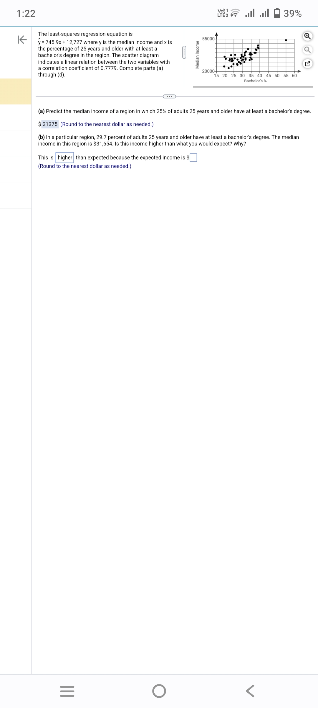
The least-squares regression equation is y=745.9x + 12,727 where y is the median income and x is the percentage of 25 years and older with at least a bachelor's degree in the region. The scatter diagram indicates a linear relation between the two variables with a correlation coefficient of 0.7779. Complete parts (a) through (d). Median Income This is higher than expected because the expected income is $ (Round to the nearest dollar as needed.) 55000 20000+ 15 20 25 30 35 40 45 50 55 60 Bachelor's % √ (a) Predict the median income of a region in which 25% of adults 25 years and older have at least a bachelor's degree. $31375 (Round to the nearest dollar as needed.) (b) In a particular region, 29.7 percent of adults 25 years and older have at least a bachelor's degree. The median income in this region is $31,654. Is this income higher than what you would expect? Why?

Researchers studying tigers collected data on the length (in meters) and weight (in kilograms) of the animals. Is there statistically significant evidence that the length of tigers is related to their weight?

Develop an estimated multiple regression equation that relates risk of a stroke to a person's age, systolic blood pressure and whether the person is a smoker.  x1=persons age x2systrolic blood pressure x3=whether person is a smoker or non smoker

The table below shows the average weekly wages​ (in dollars) for state government employees and federal government employees for 10 years. Construct and interpret a 98% prediction interval for the average weekly wages of federal government employees when the average weekly wages of state government employees is​ $878.The equation of the regression line is y=1.342x+55.816. Wages [state]- 712, 746, 786, 803, 841, 879, 918, 926, 954, 979 Wages [federal]- 1,024, 1,048, 1,098, 1,135, 1,195, 1,240, 1,270, 1,299, 1,340, 1,376 Construct and interpret a 98​% prediction interval for the average weekly wages of federal government employees when the average weekly wages of state government employees is $878. Select the correct choice below and fill in the answer boxes to complete your choice. (Round to the nearest cent as​ needed.)     PICK THE CORRECT ANSWER [A] We can be 98​% confident that when the average weekly wages of state government employees is $878​, the average weekly wages of…

The table below shows the average weekly wages (in dollars) for state government employees and federal government employees for 10 years, construct and interpret a 98% prediction interval for the average weekly wages of federal government employees when the average weekly wages of state government employees is $888 the equation of the regression line is y= 1.453x-47.386. Wages(state), X | 739|760|784|822|898|921|937|954|965| Wages (federal), Y |1,036|1,054|1,105|1,136|1,192|1,253|1,266|1,327|1,400|

I need help with this last part of this exercise.

The data show the chest size and weight of several bears. Find the regression​ equation, letting chest size be the independent​ (x) variable. Then find the best predicted weight of a bear with a chest size of 58 inches. Is the result close to the actual weight of 572 ​pounds? Use a significance level of 0.05.   Chest size​ (inches) 46 57 53 41 40 40   Weight​ (pounds) 384 580 542 358 306 320   LOADING... Click the icon to view the critical values of the Pearson correlation coefficient r. What is the regression​ equation?   y=nothing+nothingx ​ (Round to one decimal place as​ needed.)

The table shows a part of an output of a linear regression model predicting the average fare on different flight routes. Data Table Regression Table Coefficient Constant 95.80976147 COUPON −9.61654124 DISTANCE 0.080733811 PAX −0.000167343 What is the difference in prediction of the following two routes? Route A that is 3,000 miles, with COUPON=1.5 and PAX=6,000 Route B that is 3,000 miles, with COUPON=1.2 and PAX=6,000.

If a correlation isr= 0.00, then SP = 0 and the regression equation is O Ý =X +0 O Ý =X + X O Ý =0 + X O Ý =Ÿ + 0

State whether the slope of a simple linear regression line is statistically significant, then the correlation will also always be significant?