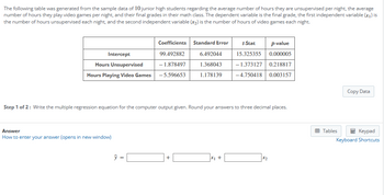
The following table was generated from the sample data of 10 junior high students regarding the average number of hours they are unsupervised per night, the average number of hours they play video games per night, and their final grades in their math class. The dependent variable is the final grade, the first independent variable (x1) is the number of hours unsupervised each night, and the second independent variable (2) is the number of hours of video games each night. Intercept Coefficients Standard Error 99.492882 t-Stat 6.492044 Hours Unsupervised Hours Playing Video Games -1.878497 -5.596653 1.368043 1.178139 p-value 15.325355 0.000005 -1.373127 0.218817 -4.750418 0.003157 Step 1 of 2: Write the multiple regression equation for the computer output given. Round your answers to three decimal places. How to enter your answer (opens in new window) Answer y = + x1 + x2 Copy Data Tables Keypad Keyboard Shortcuts

q11-

The data for this question is given in the file 1.Q1.xlsx(see image)  and it refers to data for some cities X1 = total overall reported crime rate per 1 million residents X3 = annual police funding in $/resident X7 = % of people 25 years+ with at least 4 years of college   (a) Estimate a regression with X1 as the dependent variable and X3 and X7 as the independent variables. (b) Will additional education help to reduce total overall crime (lead to a statistically significant reduction in crime)? Please explain. (c) Will an increase in funding for the police departments help reduce total overall crime (lead to a statistically significant reduction in total overall crime)? Please explain. (d) If you were asked to recommend a policy to reduce crime, then, based only on the above regression results, would you choose to invest in education (local schools) or in additional funding for the police? Please explain.

For each of the following scenarios, indicate whether the relationship between the two variables is positive or negative, as well as which line on the previous graph has a slope that reflects this type of relationship.   Hint: The X-axis and Y-axis on the graph are not labeled intentionally. You need to substitute the variables from each scenario for the horizontal and vertical axis. For example, in the first scenario, X-axis should be labeled “ ice-cream" and Y-axis should be labeled "The temperature". Relationship options: positive, negative Line options: A, B, C, D   True or False: Line D has a slope of infinity.

The following table was generated from the sample data of 10 college students regarding the number of parking tickets the student receives in a semester, the student's age, and the student's GPA. The dependent variable is the student's GPA, the first independent variable (x1) is the number of parking tickets, and the second independent variable (x2) is the student's age. Intercept Coefficients Standard Error 15.034003 1.302739 1-Stat p-value 11.540305 0.000025 Number of Parking Tickets -0.026275 0.030254 Student's Age -0.638331 0.062922 -0.868470 0.418515 -10.144838 0.000053 Copy Data Step 1 of 2: Write the multiple regression equation for the computer output given. Round your answers to three decimal places. Answer How to enter your answer (opens in new window) + x + x2 Tables Keypad Keyboard Shortcuts

You are given information on the use of public transportation in the data set within the image. Number of weekly riders                                     y -variable Price per week (of using public transportation) x-variable Population of city                                                 x-variable Monthly income of riders                                     x variable         Average parking rates per month x-variable   (a) Run a regression of the Number of weekly riders on Price per week, Population of city, Monthly income of riders, Average parking rates per month. Please copy and paste your regression results and do not submit your EXCEL worksheet.   (b) If the average parking rates increase by $1, what will be the change in the number of weekly riders? Will this change be a statistically significant change? Please explain.   (c) If the price per week (of using public transportation) increases by $1, what will be the change in the number of weekly riders? Will this change be…

Use a software of your own choice to calculate the daily log prices (lp) and daily log returns (Ir) i. Examine the descriptive statistics of both lp and Ir. What do you conclude about the distributions of lp and Ir? Is lp normally distributed? Is Ir normally distributed? Obtain the correlograms, and examine the autocorrelations and partial autocorrelations for both lp and Ir. What do you conclude about the behaviour of lp and Ir? Are they stationary/non-stationary? ii. iii. Are your conclusions about stationary/non-stationary of lp and lr confirmed by appropriate unit root tests?

A marketing analyst wants to examine the relationship between sales (in $1,000s) and advertising (in $100s) for firms in the food and beverage industry and so collects monthly data for 25 firms. He estimates the model: Sales 6g + 61 Advertising + e. The following table shows a portion of the regression results. Coefficients Standard Error t-stat p-value 40.10 14.88 2.848 0.0052 Intercept Advertising 2.88 1.52 -1.895 0.0608 When testing whether Advertising is significant at the 10% significance level, the conclusion is to Multiple Choice reject Hg, we can conclude advertising is significant not reject He; we cannot conclude advertising is significant reject He; we cannot conclude advertising is significant not reject He; we can conclude advertising is significant

solve within 30 mins.

RQ7. A teacher is trying to predict student test grades (Q). She believes test grades are a function of incoming GPA, hours studying, and hours spent on social media (a distraction). She runs a regression and it produces these coefficients: Variable Coefficient Intercept GPA Hours Studying Social Media 70.0 3.5 2.4 -4.0 For a given student Julian, his GPA is 2.0, he studies 4 hours for the exam, and he spends 6 hours on Facebook. Predict his exam score (round to the nearest whole number).