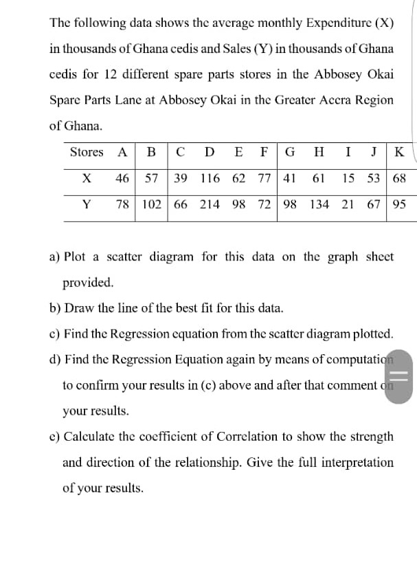
The following data shows the average monthly Expenditure (X) in thousands of Ghana cedis and Sales (Y) in thousands of Ghana cedis for 12 different spare parts stores in the Abbosey Okai Spare Parts Lane at Abbosey Okai in the Greater Accra Region of Ghana. Stores A в |сDEF G H I к X 46 57 39 116 62 77 41 61 15 53 68 Y 78 102 66 214 98 72 98 134 21 67 95 a) Plot a scatter diagram for this data on the graph sheet provided. b) Draw the line of the best fit for this data. c) Find the Regression equation from the scatter diagram plotted. d) Find the Regression Equation again by means of computation to confirm your results in (c) above and after that comment on your results. e) Calculate the coefficient of Correlation to show the strength and direction of the relationship. Give the full interpretation of your results.

1. The information in the following table shows the amount of sales and the profit from a small retail business in Whitby Ontario for the last 15 years. The years have not been provided as you will only need the amounts. Sales ($) (thousands) Profit ($) (thousands) 195 10 205 15 225 22 240 -10 255 25 300 39 265 24 345 55 295 32 335 37 380 48 405 55 355 50 390 48 410 55 a) Create a scatter plot of the data. Identify any outliers, if they occur. b) Sketch the line of best fit and determine its equation. A c) Describe any correlation you see between the variables. What conclusion could someone make based on the scatter plot? ( d) Identify whether you would use interpolation or extrapolation to predict the profit for the sales amount $500,000 and $230,000. e) Predict the profit for the sales amount $500,000 and $230,000.

The following table lists highway miles (in MPG) and weight (in pounds) for a variety of cars, foreign and domestic (same data as before). CAR HWY WEIGHT Chev. Cavalier 31 2795 Lincoln Cont. 24 3930 Mitsubishi Eclipse 33 3235 Olds. Aurora 26 3995 Pontiac Grand Am 30 3115 Chev. Corvette 28 3220 BMW 3-Series 27 3225 Ford Crown Victoria 24 3985 Hyundai Accent If we let x be the weight and y be the Highway MPG, and we used Excel to compute the equation of the Least- 37 2290 Square regression line (which comes out to be y = -0.00672'x + 51.1156) as well as the correlation coefficient (which comes out to be -0.89). Then you used that equation to predict that the Highway Miles for a car that weighs just 1000 pounds would be 44.4 mpg. I think this prediction is accurate because the person used Excel for the computation. O I think this prediction is not accurate since a car that weighs 1000 pounds is not part of the original data list. O Ithink this prediction is not accurate because the person…

.The two data sets below represent the high temperatures in two citieseach day for 5 days.City A: 18°F, 44°F, 52°F, 55°F, 58°F, 56°FCity B: 15°F, 41°F, 63°F, 61°F, 57°F, 60°F Which statementbestdescribes the measure of center that provides themost accurate estimation of the high temperature in a day in each city? A.mean, because there is an even number of values in each data set B.median, because there is an even number of values in each data set C.mean, because there is one value in each data set that is significantlylower than the other values D.median, because there is one value in each data set that issignificantly lower than the other values

2) Let x represent the average annual hours per person spent in traffic delays and y represent the average annual gallons of fuel wasted per person in traffic delays. A random sample of 8 cities showed the following data: X Y 28 jo 48 5 12 3 20 34 35 ZD 25 20 34 23 30 35 40 38 18 a) Draw a scatter plot diagram and the line that you think that best fits the data 60%" so: Ave Gallons 40 30 28 5 Five. Hours Delay 9 b) Would you say the correlation is positive, negative or close to zero?

A high school has 44 players on the football team. The summary of the players' weights is given in the box plot. Approximately, what is the percentage of players weighing greater than or equal to 245 pounds? 191 217 245 164 262 - 0o 150 160 170 180 190 200 210 220 230 240 250 260 270 00 Weight unds) Answer E Tables E Keypad Keyboard Shortcuts % Submit Answer © 2022 Hawkes Learning

3. Using data in question 6, determine whether there is enough evidence to conclude that the type II has higher strength than type I? Use a pooled t-test with a = 0.05. 1. Identify the parameters 2. Null Hypothesis 3. Alternative Hypothesis 4. Test Statistic 5. Rejection Region 6. Conclusion