
MATLAB: An Introduction with Applications
6th Edition
ISBN: 9781119256830
Author: Amos Gilat
Publisher: John Wiley & Sons Inc
expand_more
expand_more
format_list_bulleted
Related questions
Concept explainers
Topic Video
Question
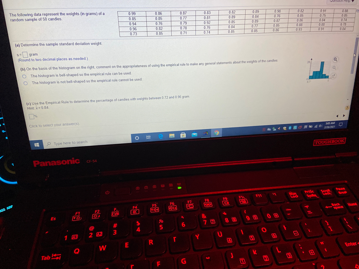

Transcribed Image Text:The following data represent the weights (in grams) of a
random sample of 50 candies.
Question Heip
0.99
0.86
0.85
0.76
0.87
0,7
0.79
0.78
0.71
0.83
0.81
0.82
0.89
0.98
0.76
0.89
0.84
0.89
0.77
0.85
0.82
0.85
0.86
0.91
0.85
0.94
0.96
0.88
0.75
0.92
0.76
0.74
0.85
0.74
0.78
0.84
0.85
0.84
0.87
0.85
0.86
0.84
0.82
0.85
0.88
0.88
0.93
0.73
0.85
0.91
(a) Determine the sample standard deviation weight
s= gram
(Round to two decimal places as needed.)
(b) On the basis of the histogram on the right, comment on the appropriateness of using the empirical rule to make any general statements about the weights of the candies
The histogram is bell-shaped so the empirical rule can be used.
The histogram is not bell-shaped so the empirical rule cannot be used.
(c) Use the Empirical Rule to determine the percentage of candies with weights between 0.72 and 0.96 gram
Hint x=0.84.
Click to select your answer(s).
505 AM
イ電 國口月知威中
2/26/2021
P Type here to search
TOUGHBOOK
Panasonic C-54
NO
Pause
Scroll
Lock
bysks
PrtSc
F11
Nun
Lock
Break
F8
F9
F1
ASS AIRP
F7
F5
F6
F.
F4
F1
F2
Back
space
Home
Es
%3D
@
4
1 AI
2 42
Y
E
5
Q
W
Tab
Enter
G
2
日
田
F
---
~の

Transcribed Image Text:The following data represent the weights (in grams) of a
random sample of 50 candies.
Question Help ▼
0.99
0.86
0.85
0.76
0.82
0.85
0.87
0.83
0.82
0.89
0.84
0.89
0.98
0.76
0.82
0.85
0.86
0.88
0.93
0.85
0.94
0.77
0.81
0.89
0.91
0.88
0.75
0.85
0.79
0.78
0.71
0.92
0.76
0.74
0,85
0.87
0.85
0.86
0.96
0.84
0.74
0.84
0.77
0.85
0.73
0.88
0.78
0.85
0.91
0.84
(c) Use the Empirical Rule to determine the percentage of candies with weights between 0.72 and 0.96 gram.
Hint: x=0.84
口%
(d) Determine the actual percentage of candies that weigh between 0.72 and 0.96 gram, inclusive.
%
(e) Use the Empirical Rule to determine the percentage of candies with weights more than 0.9 gram
%
(f) Determine the actual percentage of candies that weigh more than 0.9 gram.
Click to select your answer(s)
506 AM
A 0 A 2/26/2021
耳中
P Type here to search
TOUGHBOOK
Panasonic
CF-54
CO
Nun
Lock
PrtSc
SysRa
bysds
Scrol
Lock
Pause
Break
F1L
F11
11
F8
F9
ASS AIRBA
F7
F5
F6
F.
F4
lol
F1
F2
Back
space
Es
Home
&
23
8 B
2 A2
Page
Ur
1 41
E
5
W
Tab
Enter
K.
G
13
田
S
AShift
A4
Expert Solution
This question has been solved!
Explore an expertly crafted, step-by-step solution for a thorough understanding of key concepts.

This is a popular solution

Trending nowThis is a popular solution!

Step by stepSolved in 3 steps

Knowledge Booster


Learn more about
Need a deep-dive on the concept behind this application? Look no further. Learn more about this topic, statistics and related others by exploring similar questions and additional content below.Similar questions
- W Use the accompanying radiation levels in for 50 kg different cell phones. Find the percentile P70- 0.20 0.26 0.30 0.44 0.61 0.62 0.63 0.70 0.71 0.85 0.87 0.87 0.92 0.92 0.93 0.95 0.98 0.99 1.07 1.10 1.10 1.11 1.13 1.13 1.13 1.14 1.14 1.15 1.22 1.24 1.24 1.24 1.25 1.25 1.25 1.30 1.31 1.31 1.32 1.32 1.34 1.35 1.39 1.40 1.40 1.42 1.45 1.47 1.47 1.50 W (Type an integer or decimal rounded to two decimal places as needed.) P70 = ☐ kgarrow_forwardThe table below shows the frequency distribution of the weights (in grams) of pre-1964 quarters. Weight (g) 6.000-6.049 6.050-6.099 6.100-6.149 6.150-6.199 6.200-6.249 6.250-6.299 6.300-6.349 6.350-6.399 Frequency 2 1 3 8 11 11 6 5 1 Use the frequency distribution to construct a histogram. Does the histogram appear to depict data that have a normal distribution? Why or why not? O A. OB. O C. ouenbel Frequency 10- Aauenbes; 6 15 5- 0 6 20₁ 15- 10- 5- 0- 6 6.1 6.2 6.3 Weight (grams) 6.1 6.2 6.3 Weight (grams) 6.1 6.2 6.3 Weight (grams) 6.4 Q 6.4 5 Q Q Does the histogram appear to depict data that have a normal distribution? OA. The histogram appears to depict a normal distribution. The frequencies generally increase to a maximum and then decrease, and the histogram is roughly symmetn OB. The histogram does not appear to depict a normal distribution. The frequencies generally decrease to a minimum and then increase, and the histogram is roughly symmetric. OC. The histogram appears to…arrow_forwardCan someone explain question 1 (a & b), please.arrow_forward
- The following data set is composed of incidence rates of Kaposi’s sarcoma in 20 different regions of Tanzania. Reported in cases/million/year. 6.1, 6.6, 6.4, 6.6, 6.6, 7.6, 8.4, 8.5, 6.2, 7.6, 8.0, 7.3, 8.4, 6.6, 5.2, 6.2, 6.5, 5.8, 6.0, 6.1 Let μ be the true incident rate of Kaposi’s sarcoma in Tanzania is cases/million/year. If the true incident rate of Kaposi’s sarcoma in the United States is 6 cases/million/year based on a nationwide surveillance in 2014. Test whether the rate of Kaposi’s sarcoma in Tanzania is different from the United States at the 0.05 significance level. Be sure to state the null and alternative hypothesis. Carry out the appropriate hypothesis test by hand (you can also use SAS) and report the test statistic and the p-value and your conclusion in the context of the problem. What assumptions do we need for the validity of this hypothesis test?arrow_forward8.88. 16.0 18.0 20.0 22.0 24.0 26.0 28.0 30.0 32.0 34.0 36.0 38.0 40.0 42.0 44.0 MPGCity a) How many hatchbacks get 23 mpg in the city? Describe the distribution of the dotplot. b) What is/are the mpg rate(s) that occur most frequently? c) Which mpg rate is the middle rate (this measure of center is typically called the median)? What is the mean mpg? d) Take the data from the dotplot to create a boxplot, stem-and-leaf plot, and histogram. You must use software, such as StatCrunch or the Art of Stat to create your graphs.arrow_forwardA statistical program is recommended. A paper gave the following data on n = 11 female black bears. Age(years) Weight(kg) Home-RangeSize (km2) 10.5 54 43.0 6.5 40 46.6 28.5 62 57.4 6.5 55 35.7 7.5 56 62.0 6.5 62 33.8 5.5 42 39.7 7.5 40 32.3 11.5 59 57.2 9.5 51 24.3 5.5 50 68.6 (a) Fit a multiple regression model to describe the relationship between y = home-range size and the predictors x1 = age and x2 = weight. (Round your numerical values to four decimal places.) = (b) If appropriate, carry out a model utility test with a significance level of 0.05 to determine if at least one of the predictors age and weight is useful for predicting home range size. State the null and alternative hypotheses. H0: ?1 = ?2 = 1Ha: at least one of ?1 or ?2 is not 1.H0: At least one of ?1 or ?2 is not 1.Ha: ?1 = ?2 = 1 H0: ?1 = ?2 = 0Ha: at least one of ?1 or ?2 is not 0.H0: At least one of ?1 or ?2 is not 0.Ha: ?1 = ?2 = 0 Calculate the test…arrow_forward
- Here are the weights in ounces of a random sample of 25 oranges harvested at Sunny Day Orchards this season. 12.6 10.0 11.4 13.6 12.8 8.0 9.7 10.1 9.5 7.1 9.0 9.3 6.5 15.9 7.4 14.1 5.1 8.8 4.9 8.1 10.8 7.5 4.6 10.1 10.2 Interpret the confidence interval in the context of the problem. 3 Previous BI U AAI EE X X, EE 12pt DELL Paragraph f E Next Darrow_forwardA sample of rental cars showed the following annual mileage (in thousands of miles) 46.768 34.813 69.194 36.927 57.666 36.003 42.961 37.194 47.750 41.738 44.239 34.052 31.731 54.661 30.928 47.847 31.286 38.813 40.166 32.905 42.057 49.834 47.556 37.729 22.120 40.822 41.104 62.399 32.550 43.558 8 The sum of x is, a 1147.569 b 1183.061 c 1219.650 d 1257.371arrow_forwardThe accompanying data below represent the miles per gallon of a random sample of cars with a three-cylinder, 1.0 liter engine. 32.7 35.7 38.0 38.7 40.2 42.1 34.1 36.4 38.1 39.1 40.6 42.9 34.5 37.4 38.3 39.5 41.4 43.4 35.6 37.7 38.6 39.6 41.6 48.9 Compute the z-score corresponding to the individual who obtained 37.4 miles per gallon. Interpret this result. The z-score corresponding to the individual is ____ and indicates that the data value is _____ standard deviation(s) above/below the mean/median (Type integers or decimals rounded to two decimal places as needed.)arrow_forward
arrow_back_ios
arrow_forward_ios
Recommended textbooks for you
- MATLAB: An Introduction with ApplicationsStatisticsISBN:9781119256830Author:Amos GilatPublisher:John Wiley & Sons Inc
 Probability and Statistics for Engineering and th...StatisticsISBN:9781305251809Author:Jay L. DevorePublisher:Cengage Learning
 Statistics for The Behavioral Sciences (MindTap C...StatisticsISBN:9781305504912Author:Frederick J Gravetter, Larry B. WallnauPublisher:Cengage Learning
  Elementary Statistics: Picturing the World (7th E...StatisticsISBN:9780134683416Author:Ron Larson, Betsy FarberPublisher:PEARSON
 The Basic Practice of StatisticsStatisticsISBN:9781319042578Author:David S. Moore, William I. Notz, Michael A. FlignerPublisher:W. H. Freeman
 Introduction to the Practice of StatisticsStatisticsISBN:9781319013387Author:David S. Moore, George P. McCabe, Bruce A. CraigPublisher:W. H. Freeman
MATLAB: An Introduction with Applications
Statistics
ISBN:9781119256830
Author:Amos Gilat
Publisher:John Wiley & Sons Inc
Probability and Statistics for Engineering and th...
Statistics
ISBN:9781305251809
Author:Jay L. Devore
Publisher:Cengage Learning
Statistics for The Behavioral Sciences (MindTap C...
Statistics
ISBN:9781305504912
Author:Frederick J Gravetter, Larry B. Wallnau
Publisher:Cengage Learning
Elementary Statistics: Picturing the World (7th E...
Statistics
ISBN:9780134683416
Author:Ron Larson, Betsy Farber
Publisher:PEARSON
The Basic Practice of Statistics
Statistics
ISBN:9781319042578
Author:David S. Moore, William I. Notz, Michael A. Fligner
Publisher:W. H. Freeman
Introduction to the Practice of Statistics
Statistics
ISBN:9781319013387
Author:David S. Moore, George P. McCabe, Bruce A. Craig
Publisher:W. H. Freeman