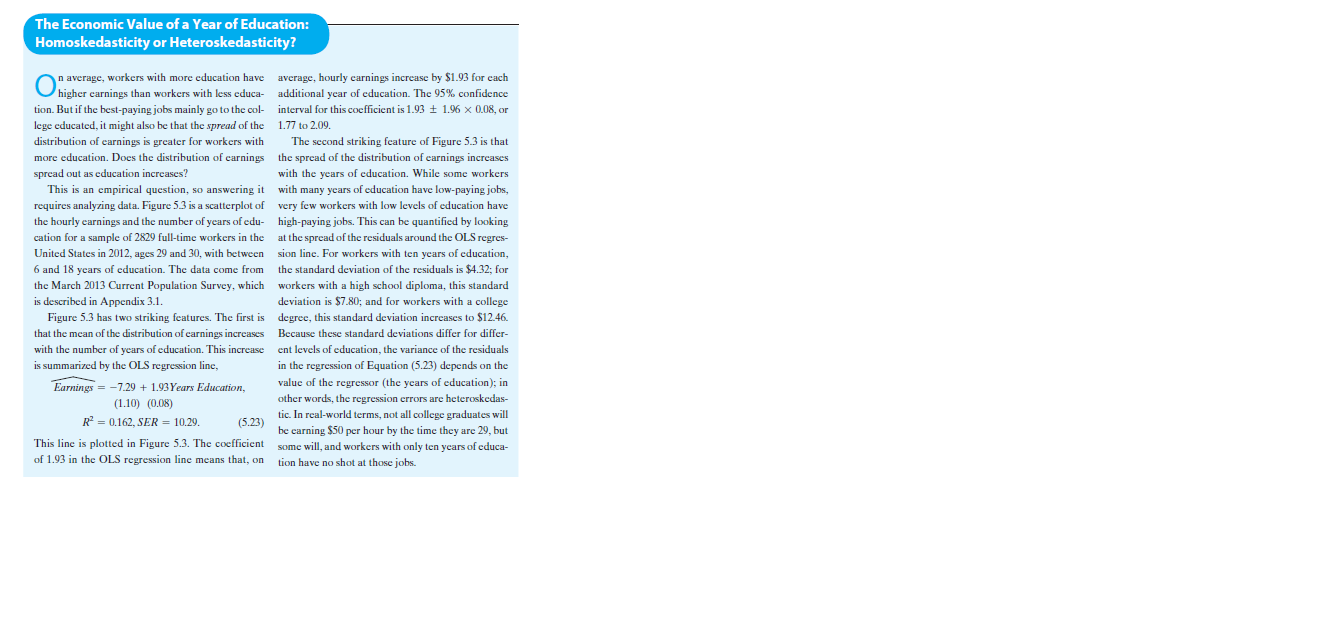
The Economic Value of a Year of Education: Homoskedasticity or Heteroskedasticity? On average, workers with more education have average, hourly carnings increase by $1.93 for cach Ohigher carnings than workers with less cduca- additional year of education. The 95% confidence tion. But if the best-paying jobs mainly go to the col- interval for this coefficient is 1.93 + 1.96 x 0.08, or lege educated, it might also be that the spread of the 1.77 to 2.09. distribution of carnings is greater for workers with The second striking feature of Figure 5.3 is that more education. Docs the distribution of carnings the spread of the distribution of earnings increases with the years of education. While some workers This is an empirical question, so answering it with many years of education have low-paying jobs, spread out as education increases? requires analyzing data. Figure 5.3 is a scatterplot of very few workers with low levels of education have the hourly carnings and the number of ycars of edu- high-paying jobs. This can be quantified by looking at the spread of the residuals around the OLS regres- cation for a sample of 2829 full-time workers in the United States in 2012, ages 29 and 30, with between n sion line. For workers with ten years of education, 6 and 18 years of education. The data come from the standard deviation of the residuals is $4.32; for the March 2013 Current Population Survey, which workers with a high school diploma, this standard is described in Appendix 3.1. Figure 5.3 has two striking features. The first is degree, this standard deviation increases to $12.46. deviation is $7.80; and for workers with a college that the mean of the distribution of carnings increases Because these standard deviations differ for differ- with the number of years of education. This increase ent levels of education, the variance of the residuals is summarized by the OLS regression line, in the on the regression of Equation (5.23) depends value of the regressor (the years of education); in Earnings = -7.29 + 1.93Years Education, (1.10) (0.08) other words, the regression errors are heteroskedas- tic. In real-world terms, not all college graduates will R = 0.162, SER = 10.29. (5.23) be carning $50 per hour by the time they are 29, but This line is plotted in Figure 5.3. The coefficient of 1.93 in the OLS regression line means that, on some will, and workers with only ten years of educa- tion have no shot at those jobs.

Prices and mileage of 48 Dodge 2500 Pickup trucks with Cummins diesel engines.  Prices ranged from $28,925 to $68,650.  Mileage ranged from 315 to 186,466.   While I did not share the trucks were 2013 to 2020 models. Please show all work.  Interpret b0 in the context of this problem.  Interpret b1 in the context of this problem.  What percent of total variation in prices is explained by the regression model?  Provide evidence to support your answer. Price Mileage 52293 34450 50987 23372 62988 21738 37500 81176 66000 23118 47601 71143 47750 18214 42000 32303 50987 23372 28925 143737 42050 58561 51738 9691 51500 23969 44988 48781 29500 114809 46975 16918 63999 15507 46975 16918 43222 50459 38386 87192 42000 68722 62250 14042 62998 21738 32130 103644 52293 34450 52900 68883 53172 3656 53494 315 39594 88441 63246 23631 58250 34974 59391 18383 50650 42737 54976 84200 68650 14401 51114 47433 43900 74106 37450…

Suppose a new location opens in an area with a population of 144,000, an average income of$36,000, an average age of 27, and $2,000 spent on advertising in the previous month.a. Use your chosen regression to predict Gross Sales for the month at the new location. (I picked population)b. Suppose actual Gross Sales for the month were $420,624. Does this make sense,given your model and predicted value?12. Using your chosen regression model,a. Identify the slope and explain what it means, in the context of the model.b. Identify the initial value or y-intercept and explain what it means, in the context ofthe model.

50

2. Participants were kept awake for a certain number of hours before given a visuospatial task. Researchers measured how many correct responses each participant had. Results are shown below. Use alpha = .01. Number of Correct Hours Kept Awake (X) Responses (Y) 21 X = 10 SS, = 422 Y = 10 SS, = 690 2 4 19 %3D 6. 13 SPxy =-525 ху 5 20 S, =5.70 S, = 7.29 9. 11 10 9. 14 5 15 5 17 2 18 1 17 1 13 4 18 8 11 A. Graph the data. B. State the hypotheses. C. Make a decision about the null. a. Calculate Pearson's r i. Decision about null hypothesis? b. Calculate effect size i. Interpret effect size. D. State your conclusion. E. Relate your conclusion to the research. F. Calculate the regression formula. G. If someone was kept awake for 9 hours, what is the predicted number of correct responses?

2

Construct and interpret a​ 95% prediction interval for the proceeds when the number of issues is 658.

14

3. Regression analysis breaks scores on the DV into... (explain and give equations)

Construct and interpret a​ 95% prediction interval for the proceeds when the number of issues is 602.