
MATLAB: An Introduction with Applications
6th Edition
ISBN: 9781119256830
Author: Amos Gilat
Publisher: John Wiley & Sons Inc
expand_more
expand_more
format_list_bulleted
Related questions
Concept explainers
Topic Video
Question
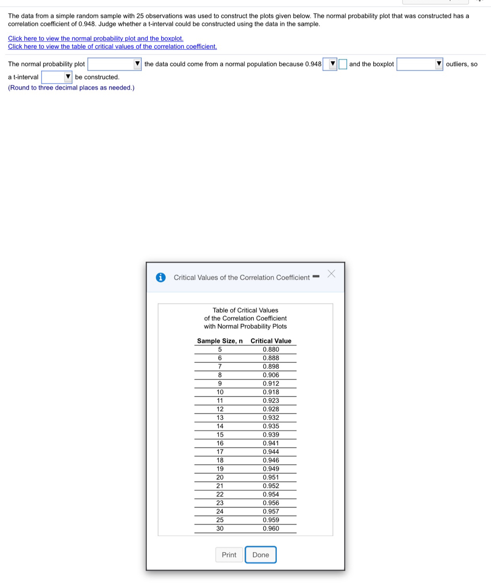

Transcribed Image Text:The data from a simple random sample with 25 observations was used to construct the plots given below. The normal probability plot that was constructed has a
correlation coefficient of 0.948. Judge whether a t-interval could be constructed using the data in the sample.
Click here to view the normal probability plot and the boxplot.
Click here to view the table of critical values of the correlation coefficient.
The normal probability plot
v the data could come from a normal population because 0.948
|and the boxplot
outliers, so
a t-interval
V be constructed.
(Round to three decimal places as needed.)
Critical Values of the Correlation Coefficient
Table of Critical Values
of the Correlation Coefficient
with Normal Probability Plots
Sample Size, n Critical Value
0.880
0.888
7
0.898
8
0.906
6.
0.912
10
0.918
11
0.923
12
0.928
13
0.932
14
0.935
15
0.939
16
0.941
17
0.944
18
0.946
19
0.949
20
0.951
21
0.952
0.954
22
23
0.956
24
0.957
25
0.959
30
0.960
Print
Done

Transcribed Image Text:Question Heip
The data from a simple random sample with 25 observations was used to construct the plots given below. The normal probability plot that was constructed has a
correlation coefficient of 0.948. Judge whether a t-interval could be constructed using the data in the sample.
Click here to view the normal probability_plot and the boxplot.
Click here to view the table of critical values of the correlation coefficient,
The normal probability plot
V the data could come from a normal population because 0.948
and the boxplot
V outliers, so
a t-interval
V be constructed.
(Round to three decimal places as needed.)
Normal Probability Plot and Bloxplot
10
20
30
40
-20
-jo
10
20
30
40
50
60
Data
Print
Done
Expected Z-Score
Expert Solution
This question has been solved!
Explore an expertly crafted, step-by-step solution for a thorough understanding of key concepts.

This is a popular solution

Trending nowThis is a popular solution!

Step by stepSolved in 2 steps

Knowledge Booster


Learn more about
Need a deep-dive on the concept behind this application? Look no further. Learn more about this topic, statistics and related others by exploring similar questions and additional content below.Similar questions
- This is only one questionarrow_forwardThe table available below shows the weights (in pounds) for a sample of vacuum cleaners. The weights are classified according to vacuum cleaner type. At a = 0.10, can you conclude that at least one mean vacuum cleaner weight is different from the others? Click the icon to view the vacuum cleaner weight data. Let μBU, BLU, and μTC represent the mean weights for bagged upright, bagless upright, and top canister vacuums respectively. What are the hypotheses for this test? A. Ho: At least one of the means is different. Ha: MBUHBLUPTC B. Ho: "BU HBLU HTC # Ha: MBUHBLUPTC C. Ho: MBUHBLU = HTC Ha: At least one of the means is different. D. Ho: MBU - HBLU = μTC Ha: HBU #BLU HTC What is the test statistic? F = 12.56 (Round to two decimal places as needed.) What is the P-value? P-value = 0.000624 (Round to three decimal places as needed.)arrow_forwardIs the variable(foot print) below normally distributed or skewed? If skewed, indicate the direction. male shoe print #1 32.2 #2 30.1 #3 29.0 #4 31.8 #5 29.4arrow_forward
- A back-to-back stem-and-leaf plot compares two data sets by using the same stems for each data set. Leaves for the first data set are on one side while leaves for the second data set are on the other side. The back-to-back stem- and-leaf plot available below shows the salaries (in thousands) of all lawyers at two small law firms. Complete parts (a) and (b) below. Click the icon to view the back-to-back stem-and-leaf plot. (a) What are the lowest and highest salaries at Law Firm A? at Law Firm B? How many lawyers are in each firm? At Law Firm A the lowest salary was $ At Law Firm B the lowest salary was $ and the highest salary was $ and the highest salary was $arrow_forwardI vacuum cleaners. The weights are classified according to vacuum cleaner type. At a=0.10, can you conclude that at least one mean vacuum cleaner weight is different The table available below shows the weights (in pounds) for a sample from the others? E Click the icon to view the vacuum cleaner weight data. Let Hgu. PBLU and PTC represent the mean weights for bagged upright, bagless upright, and top canister vacuums respectively. What are the hypotheses for this test? O A. Ho: Heu * PBLU HTC H PBU PBLU =HTC Weight of Vacuum Cleaners by Type O B. Ho: At least one of the means is different. H PBu = HBLUu =PTC &c. Họ: PBU = HBLU =HTC Bagged upright 22 19 Bagless upright Top canister 21 22 23 25 H: At least one of the means different. 17 20 15 18 18 19 O D. Ho: PBU = PBLU "HTC 23 20 26 25 22| 23 Ha: Peu * PBLU *HTC What is the test statistic? Print Done F= (Round to two decimal places as needed.)arrow_forwardA set of data has a histogram that is extremely skewed, what does this tell you about the data and how observations will tend to fall around the mean?arrow_forward
- Given the scatter plot below, which of the following describes the strength and direction of the data? 10 Weak negative correlation Strong negative correlation Strong positive correlation Weak positive correlationarrow_forwardWhat are the most likely values of r for each plot of data shown below? Figure 1 *AT THE TOP r = -0.5 r = 0 r= 0.5 r = 1 ? Answer: Figure 2 *AT THE Bottom r = -0.5 r = 0 r= 0.5 r = 1 ? Answer:arrow_forward
arrow_back_ios
arrow_forward_ios
Recommended textbooks for you
- MATLAB: An Introduction with ApplicationsStatisticsISBN:9781119256830Author:Amos GilatPublisher:John Wiley & Sons Inc
 Probability and Statistics for Engineering and th...StatisticsISBN:9781305251809Author:Jay L. DevorePublisher:Cengage Learning
 Statistics for The Behavioral Sciences (MindTap C...StatisticsISBN:9781305504912Author:Frederick J Gravetter, Larry B. WallnauPublisher:Cengage Learning
  Elementary Statistics: Picturing the World (7th E...StatisticsISBN:9780134683416Author:Ron Larson, Betsy FarberPublisher:PEARSON
 The Basic Practice of StatisticsStatisticsISBN:9781319042578Author:David S. Moore, William I. Notz, Michael A. FlignerPublisher:W. H. Freeman
 Introduction to the Practice of StatisticsStatisticsISBN:9781319013387Author:David S. Moore, George P. McCabe, Bruce A. CraigPublisher:W. H. Freeman
MATLAB: An Introduction with Applications
Statistics
ISBN:9781119256830
Author:Amos Gilat
Publisher:John Wiley & Sons Inc
Probability and Statistics for Engineering and th...
Statistics
ISBN:9781305251809
Author:Jay L. Devore
Publisher:Cengage Learning
Statistics for The Behavioral Sciences (MindTap C...
Statistics
ISBN:9781305504912
Author:Frederick J Gravetter, Larry B. Wallnau
Publisher:Cengage Learning
Elementary Statistics: Picturing the World (7th E...
Statistics
ISBN:9780134683416
Author:Ron Larson, Betsy Farber
Publisher:PEARSON
The Basic Practice of Statistics
Statistics
ISBN:9781319042578
Author:David S. Moore, William I. Notz, Michael A. Fligner
Publisher:W. H. Freeman
Introduction to the Practice of Statistics
Statistics
ISBN:9781319013387
Author:David S. Moore, George P. McCabe, Bruce A. Craig
Publisher:W. H. Freeman