
MATLAB: An Introduction with Applications
6th Edition
ISBN: 9781119256830
Author: Amos Gilat
Publisher: John Wiley & Sons Inc
expand_more
expand_more
format_list_bulleted
Related questions
Question
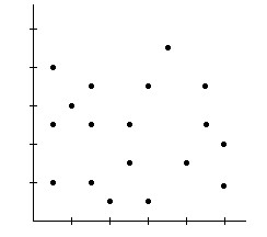
Tell what the residual plot indicates about the appropriateness of the linear model that was fit to the data.
Choose the best answer:
A. Model may not be appropriate. The spread is changing.
B. Model is not appropriate. The relationship is nonlinear.
C. Model is appropriate.

Transcribed Image Text:+
Expert Solution
This question has been solved!
Explore an expertly crafted, step-by-step solution for a thorough understanding of key concepts.

This is a popular solution

Trending nowThis is a popular solution!

Step by stepSolved in 2 steps

Knowledge Booster

Similar questions
- The table below shows the number of state-registered automatic weapons and the murder rate for several Northwestern states. I 11.7 8 6.8 3.6 2.3 2.5 2.5 0.4 y 13.7 11 9.8 I= thousands of automatic weapons 7.4 6.2 6.2 4.2 y = murders per 100,000 residents This data can be modeled by the equation y = 0.84x + 4.11. Use this equation to answer the following; Special Note: I suggest you verify this equation by performing linear regression on your calculator. Use the equation with the values rounded to two decimal places to make your predictions. A) How many murders per 100,000 residents can be expected in a state with 8.5 thousand automatic weapons? Answer = Round to 3 decimal places. B) How many murders per 100,000 residents can be expected in a state with 2.8 thousand automatic weapons? Answer Round to 3 decimal places.arrow_forwardThe table below shows the number of state-registered automatic weapons and the murder rate for several Northwestern states. 11.5 7. 11.2 8.5 3.7 2.4 2.7 2.1 0.4 13.6 10 7.5 6. 6.2 5.5 4.1 I = thousands of automatic weapons y= murders per 100,000 residents This data can be modeled by the linear equation ý = 0.86x +3.92 a. How many murders per 100,000 residents can be expected in a state with 2.2 thousand automatic weapons? Round to 3 decimal places. murders per 100,000 residents b. How many murders per 100,000 residents can be expected in a state with 6 thousand automatic weapons? Round to 3 decimal places. murders per 100,000 residents Question Help: Video Submit Questionarrow_forwardThe scatter plot shows the relationship between the number of minutes studying for a test (x) and the number of mistakes made (y). The graph shows the scatterplot of the data and a fitted line. 19+ 18 17 16 15 14 13 12 10 4 -10 10 20 30 40 50 60 70 80 90 100 lio a2 Select True or False for each statement based on the scatter plot. True/False There is a negative association between the amount of time studying for a test and the number of mistakes made. True False Students who studied for a longer period of time tended to make more mistakes. True False There is a linear association between time True False studying and number of mistakes.arrow_forward
- The table below shows the number of state-registered automatic weapons and the murder rate for several Northwestern states. x 11.8 8.2 6.8 3.5 2.8 2.8 2.3 0.5 y 13.9 10.8 10.1 7.2 6.5 6.5 6.3 4.8 x = thousands of automatic weapons y = murders per 100,000 residents This data can be modeled by the equation y = 0.81x + 4.35. Use this equation to answer the following; Special Note: I suggest you verify this equation by performing linear regression on your calculator. A) How many murders per 100,000 residents can be expected in a state with 7 thousand automatic weapons? Round to 3 decimal places. B) How many murders per 100,000 residents can be expected in a state with 7.8 thousand automatic weapons? Answer = Answer = Round to 3 decimal places.arrow_forwardBelow is a scatterplot of a student’s SAT score and their college GPA. Suppose we want to decide if a student’s SAT score and their GPA are linearly related. What does this scatterplot tell us of the relationship? Support your answer. SAT score_GPA scatterplot.pdfarrow_forwardsolve last questionarrow_forward
- Please help me better understand this problem. Researchers want to determine if heavier cars use more gasoline? To answer this question, a researcher randomly selected 15 cars. He collected their weight (in hundreds of pounds) and the mileage (MPG) for each car. From a scatterplot made with the data, a linear model seemed appropriate and the following output was obtained in photo below. Question: Determine the proportion of the variation in mileage is accounted for by the linear relationship with the weight of the car and also determine the estimate of the regression standard deviation.arrow_forwardThe data show the chest size and weight of several bears. Find the regression equation, letting chest size be the independent (x) variable. Then find the best predicted weight of a bear with a chest size of 58 inches. Is the result close to the actual weight of 572 pounds? Use a significance level of 0.05. Chest size (inches) 46 57 53 41 40 40 Weight (pounds) 384 580 542 358 306 320 LOADING... Click the icon to view the critical values of the Pearson correlation coefficient r. What is the regression equation? y=nothing+nothingx (Round to one decimal place as needed.)arrow_forwardA. run a simple regression- dependent variable is Weeks, independent variable is Age. B. run a multiple regression with dependent variable weeks and independent variable-age, married, head, manager and sales. C. Create the regular and standardized residual plots for both. Please show the tables when entering values of the regression for both the outputs and the scatter plots.arrow_forward
- The table below shows the number of state-registered automatic weapons and the murder rate for several Northwestern states. 11.8 8.5 7 3.3 2.5 2.8 2.2 0.6 14.2 11.6 10.3 7.1 6.4 6.7 6.2 4.8 thousands of automatic weapons = murders per 100,000 residents This data can be modeled by the linear equation ŷ = 0.84x + 4.33 a. How many murders per 100,000 residents can be expected in a state with 9.1 thousand automatic weapons? Round to 3 decimal places. murders per 100,000 residents b. How many murders per 100,000 residents can be expected in a state with 4.3 thousand automatic weapons? Round to 3 decimal places. murders per 100,000 residentsarrow_forward2. The table below lists the annual land-line phone cost per costumer: Year 2012 2013 2014 2015 Cost ($) a. 692 610 Find a linear regression model for this data b. Interpret the slope of the model 580 C. Predict the annual land-line phone cost per customer in 2022 495 2016 434arrow_forwardUse table and picture to solve!!! Thank you so much arrow_forward
arrow_back_ios
SEE MORE QUESTIONS
arrow_forward_ios
Recommended textbooks for you
- MATLAB: An Introduction with ApplicationsStatisticsISBN:9781119256830Author:Amos GilatPublisher:John Wiley & Sons Inc
 Probability and Statistics for Engineering and th...StatisticsISBN:9781305251809Author:Jay L. DevorePublisher:Cengage Learning
 Statistics for The Behavioral Sciences (MindTap C...StatisticsISBN:9781305504912Author:Frederick J Gravetter, Larry B. WallnauPublisher:Cengage Learning
  Elementary Statistics: Picturing the World (7th E...StatisticsISBN:9780134683416Author:Ron Larson, Betsy FarberPublisher:PEARSON
 The Basic Practice of StatisticsStatisticsISBN:9781319042578Author:David S. Moore, William I. Notz, Michael A. FlignerPublisher:W. H. Freeman
 Introduction to the Practice of StatisticsStatisticsISBN:9781319013387Author:David S. Moore, George P. McCabe, Bruce A. CraigPublisher:W. H. Freeman
MATLAB: An Introduction with Applications
Statistics
ISBN:9781119256830
Author:Amos Gilat
Publisher:John Wiley & Sons Inc
Probability and Statistics for Engineering and th...
Statistics
ISBN:9781305251809
Author:Jay L. Devore
Publisher:Cengage Learning
Statistics for The Behavioral Sciences (MindTap C...
Statistics
ISBN:9781305504912
Author:Frederick J Gravetter, Larry B. Wallnau
Publisher:Cengage Learning
Elementary Statistics: Picturing the World (7th E...
Statistics
ISBN:9780134683416
Author:Ron Larson, Betsy Farber
Publisher:PEARSON
The Basic Practice of Statistics
Statistics
ISBN:9781319042578
Author:David S. Moore, William I. Notz, Michael A. Fligner
Publisher:W. H. Freeman
Introduction to the Practice of Statistics
Statistics
ISBN:9781319013387
Author:David S. Moore, George P. McCabe, Bruce A. Craig
Publisher:W. H. Freeman