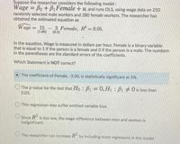
Suppose the researcher considers the following model: Wage = Bo +B1Female + u, and runs OLS, using wage data on 250 randomly selected male workers and 280 female workers. The researcher has obtained the estimated equation as Wage = 15 (1.00) 3 Female, R=0.05. (0.5) %3D %3D In the equation, Wage is measured in dollars per hour, Female is a binary variable that is equal to 1 if the person is a female and O if the person is a male. The numbers in the parentheses are the standard errors of the coefficients. Which Statement is NOT correct? The coefficient of Female, -3.00, is statistically significant at 5%. O The p-value for the test that Ho : B = 0, H, : B1 0 is less than 0.05. O This regression may suffer omitted variable bias. O Since R is too low, the wage difference between men and women is insignificant. The researcher can increase R by including more regressors in the model

The measure of standard error can also be applied to the parameter estimates resulting from linear regressions. For example, consider the following linear regression equation that describes the relationship between education and wage:   WAGEi=β0+β1EDUCi+εi   where WAGEi is the hourly wage of person i (i.e., any specific person) and EDUCiEDUCi is the number of years of education for that same person. The residual εiεi encompasses other factors that influence wage, and is assumed to be uncorrelated with education and have a mean of zero. Suppose that after collecting a cross-sectional data set, you run an OLS regression to obtain the following parameter estimates:   WAGEi=−12.3+4.4 EDUCi   If the standard error of the estimate of β1 is 1.29, then the true value of β1 lies between (2.465, 3.11, 3.755, 1.82)    and (5.69, 6.98, 5.045)   . As the number of observations in a data set grows, you would expect this range to (INCREASE OR DECREASE)    in size.

E3

please answer in text form and in proper format answer with must explanation , calculation for each part and steps clearly

Consider the following regression estimates (FN2) Linear regression belavg abvavg female married _cons b. 1 wage O C. 5 O d. 4 Robust Coef. Std. Err. 3047845 3150202 2820787 -1.063254 .0693348 -2.751963 .9686236 .2612646 6.699098 .2889831 Number of obs F(4, 1255) Prob > F R-squared Root MSE t P>|t| -3.49 0.001 0.22 0.826 -9.76 0.000 3.71 0.000 23.18 0.000 |||||||||| = = .45606 6.132155 = -1.661197 -.5486894 -3.305361 = = [95% Conf. Interval] 1,260 56.35 0.0000 0.1121 4.3987 assume that MLR 1-6 hold. In the regression above, how many coefficients (including the constant) are statistically significant at the 1% level? a. 3 -.4653108 .687359 -2.198565 1.481187 7.266042

Use matrices to solve the following pairs of simultaneous equations: 3x + 4y = -1 and 5x - y = 6

Explain the OLS Estimator in Multiple Regression in detail?

Consider the population regression of log earnings [Y;, where Y,= In(Earnings,;)] against two binary variables: whether a worker is married (D₁, where D₁;= 1 if the th person is married) and the worker's gender (D2;, where D₂;= 1 if the th person is female), and the product of the two binary variables Y₁ = Po+B₁D₁+P₂D2i + P3 (D₁¡ × D₂i) + Hi- The interaction term: O A. indicates the effect of being married on log earnings. B. does not make sense since it could be zero for married males. C. allows the population effect on log earnings of being married to depend on gender. D. cannot be estimated without the presence of a continuous variable.

Suppose we are interested in evaluating the impact on wages of being a college graduate and of residing in California. To this end we define the following dummy variables if college graduate if not college graduate coll = ncoll = if not college graduate if college graduate 1 cali = if residing in California S 1 if not residing in California ncali = if not residing in California if residing in California and for wages denoting yearly wages, we estimate the following model of returns to education wages = B1 coll+ B2ncoll + B3 cali + B4(coll x cali) + e where E[e|coll, cali] = 0. Which parameter or combination of parameters measures the increase in expected wages from obtaining a college degree (comparing to not having a college degree) when residing California? O a. None of the other options is correct O b. Bi – B2 O c. B1 – B2 + ß4 O d. B4 O e. Bi + B3 – ßi – B4 O f. Bi + B4 – ß2 – B4 Clear my choice

Find the degrees of freedom in a regression model that has 10 observations and 7 independent variables