
A First Course in Probability (10th Edition)
10th Edition
ISBN: 9780134753119
Author: Sheldon Ross
Publisher: PEARSON
expand_more
expand_more
format_list_bulleted
Related questions
Question
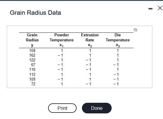

Transcribed Image Text:Grain Radius Data
Grain
Radius
y
158
162
122
67
110
112
109
72
Powder
Temperature
X₁
1
- 1
1
Print
Extrusion
Rate
X2
1
1
1
Done
Die
Temperature
X3
1
1
1
- 1
X

Transcribed Image Text:Suppose that a scientist takes experimental data on the radius of a propellant grain Y as a function of powder temperature x₁, extrusion rate
X₂, and die temperature x3. The accompanying data set is available below. Complete parts (a) and (b) below.
Click here to view the coded data.
Click here to view page 1 of the table of critical values of the t-distribution.
Click here to view page 2 of the table of critical values of the t-distribution.
(a) A case can be made for eliminating x₁, powder temperature, from the model since the P-value based on the F-test is 0.3488 while
P-values for X₂ and x3 are near zero. Reduce the model by eliminating x₁, thereby producing a full and a restricted (or reduced) model, and
compare them on the basis of R²
adj
The full model is ŷ = 127.50 + (1.25) x₁ + (18.25) x₂ + (26.25¹) x3.
(Round to two decimal places as needed.)
The restricted model is ŷ= 127.50 + (18.25¹) x₂ + (26.25) X3.
(Round to two decimal places as needed.)
For the full model, R² = 0.991, for the restricted model, R²
adj
adj
model.
a small advantage when using the full
(Round to three decimal places as needed.)
=
0.990, so there appears to be
(b) Compare the full and restricted models using the width of the 95% prediction intervals on a new observation. The better of the two models
would be that with the tightened prediction intervals. Use the average of the width of the prediction intervals.
For the full model, the average width is 22.68. For the restricted model, the average width is 20.35. So, the model without x, appears to
be the better model.
(Round to two decimal places as needed.)
Expert Solution
This question has been solved!
Explore an expertly crafted, step-by-step solution for a thorough understanding of key concepts.

Step by stepSolved in 5 steps with 11 images

Knowledge Booster

Similar questions
- Suppose u, and u, are true mean stopping distances at 50 mph for cars of a certain type equipped with two different types of braking systems. The data follows: m = 5, x = 115.1, s, = 5.05, n = 5, y = 129.2, and s, = 5.36. Calculate a 95% CI for the difference between true average stopping distances for cars equipped with system 1 and cars equipped with system 2. (Round your answers to two decimal places.) n USE SALT Does the interval suggest that precise information about the value of this difference is available? O Because the interval is so narrow, it appears that precise information is available. o Because the interval is so wide, it appears that precise information is not available. o Because the interval is so narrow, it appears that precise information is not available. Because the interval is so wide, it appears that precise information is available. You may need to use the appropriate table in the Appendix of Tables to answer this question.arrow_forwardSuppose a researcher wants to see if the proportion of college educated adults is higher in New York compared to Florida. The researcher randomly samples 500 adults in New York and found that 196 had a college education, while a random sample of 600 adults in Florida found that 227 had a college education.At the 0.05 level of significance, does the data provide evidence to suggest the proportion of college educated adults is higher in New York than Florida? Step 1: Define the parameter & setup the testStep 2: State the Level of SignificanceStep 3: Find the value of the Test StatisticsStep 4: Find P-Value OR Find Critical ValueStep 5: State Conclusion and whyarrow_forwardiris is a built-in R data set (data frame). This data set contains gives the measurements in centimeters of the variables sepal length and width and petal length and width, respectively, for 50 flowers from each of 3 species of iris. The species are Iris setosa, versicolor, and virginica. We are interested in some descriptive statistics related to the Sepal.Width column of the data frame. We can access the data directly by using the assignment x <- iris$Sepal.Width (In R use ?iris for info on this dataset.)Remember: x <- iris$Sepal.Widtha.Calculate the sample median of x. b. Using the R quantile function, find the .80 quantile of x.(80th percentile) c. Calculate the interquartile range of x using R. d. Calculate the sample mean of x. e. Calculate a 4% trimmed mean for x. f. Calculate the sample variance of x. g. Calculate the sample standard deviation of x. h. What proportion of the x values are within 2.0 sample standard deviations from the sample mean i. Calculate the minimum…arrow_forward
- The accompanying data represent the total compensation for 12 randomly selected chief executive officers (CEOS) and the company's stock performance. Use the data to complete parts (a) through (d). E Click the icon to view the data table. (a) Treating compensation as the explanatory variable, x, use technology to determine the estimates of Bo and B,- The estimate of B, is (Round to three decimal places as needed.) Data Table of Compensation and Stock Performante Compensation Company (millions of dollars) Return (%) O Stock A 14.71 75.73 В 4.02 64.29 C 6.55 141.81 D 1.32 30.73 1.73 10.75 2.43 29.05 12.26 0.56 7.07 66.32 9.51 56.31 J 3.83 58.48 K 21.29 21.52 6.63 31.85 Print Donearrow_forwardWrinkle recovery angle and tensile strength are the two most important characteristics for evaluating the performance of crosslinked cotton fabric. An increase in the degree of crosslinking, as determined by ester carboxyl band absorbance, improves the wrinkle resistance of the fabric (at the expense of reducing mechanical strength). The accompanying data on x = absorbance and y = wrinkle resistance angle was read from a graph in the paper "Predicting the Performance of Durable Press Finished Cotton Fabric with Infrared Spectroscopy".t x 0.115 0.126 0.183 0.246 0.282 0.344 0.355 0.452 0.491 0.554 0.651 y 334 342 355 363 365 372 381 400 392 412 420 Here is regression output from Minitab: Predictor Constant absorb S = 3.60498 Coef 321.878 156.711 SOURCE Regression Residual Error Total R-Sq= 98.5% DF SE Coef 2.483 6.464 1 9 10 SS 7639.0 117.0 7756..0 T 129.64 24.24 P 0.000 0.000. R-Sq (adj) 98.3% MS 7639.0 13.0 F 587.81 (a) Does the simple linear regression model appear to be appropriate?…arrow_forwardNo tortilla chip aficionado likes soggy chips, so it is important to find characteristics of the production process that produce chips with an appealing texture. The following data on x = frying time (sec) and y = moisture content (%) appeared in an article. x 5 10 15 20 25 30 45 60 y 16.4 9.7 8.1 4.2 3.3 2.8 2.0 1.2 (a) Construct a scatter plot of y versus x. y 15 10- 5 y 15 O 10 10 20 30 40 50 5 10 20 10 NE X 50 60 30 60 40 X 15 y 10 O 5 O y 15 10 20 30 40 50 60 10 20 30 Comment. The plot has a curved pattern. A linear model would not be appropriate. O The plot has a curved pattern. A linear model would be appropriate. O The plot does not have a curved pattern. A linear model would be appropriate. O The plot does not have a curved pattern. A linear model would not be appropriate. 40 50 60 X Xarrow_forward
- Q1: The data points below are related to a chemi-thermo-mechanical pulp from mixed density hardwoods. They relate Y (specific surface area of the fibres in cm/g) to the % NaOH (sodium hydroxide) used as a pretreatment chemical and the treatment time (min) for different batches of pulp. The variables are present at three different levels. In this case, it is preferred (for reasons that we will discuss later in the course) to code the levels as shown in the last two columns of the table below, designated by Xı and X2. Y SODIUM ΤΙME Xi X2 HYDROXIDE 5.95 3 30 -1 5.60 3 60 -1 5.44 3 90 -1 1 6.22 9. 30 -1 5.85 9 60 5.61 9. 90 1 8.36 15 30 1 -1 7.30 15 60 1 6.43 15 90 1 1 a. Using the variables Y, X1 and X2 (not actual time and sodium hydroxide! You will see why later!), fit the following multiple linear regression model to the data: (Model A) Y = (b0) + (b1) X1 + (b2) X2; subsequently, estimate the parameters and examine the residual plot (residuals vs Y hat). What does this residual plot…arrow_forwardpan's high population density has resulted in a multitude of resource-usage problems. One especially serious difficulty concerns waste removal. An article reported the development of a new compression machine for processing sewage sludge. An important part of the investigation involved relating the moisture content of compressed pellets (y, in %) to the machine's filtration rate (x, in kg-DS/m/hr). The following data was read from a graph in the article. x 125.8 98.1 201.4 147.3 145.9 124.7 112.2 120.2 161.2 178.9 159.5 145.8 75.1 151.5 144.2 125.0 198.8 133.9 y 77.9 76.8 81.5 79.8 78.2 78.3 77.5 77.0 80.1 80.2 79.9 79.0 76.9 78.2 79.5 78.1 81.5 71.0 (a) Determine the slope and intercept of the estimated regression line. (Round your answers to 5 decimal places, if needed.)slope: intercept: (b) Does there appear to be a useful linear relationship? Carry out a test using the ANOVA approach and a significance level of 0.05. State the appropriate null and alternative hypotheses.…arrow_forwardWrinkle recovery angle and tensile strength are the two most important characteristics for evaluating the performance of crosslinked cotton fabric. An increase in the degree of crosslinking, as determined by ester carboxyl band absorbance, improves the wrinkle resistance of the fabric (at the expense of reducing mechanical strength). The accompanying data on x = absorbance and y = wrinkle resistance angle was read from a graph in the paper "Predicting the Performance of Durable Press Finished Cotton Fabric with Infrared Spectroscopy".† x 0.115 0.126 0.183 0.246 0.282 0.344 0.355 0.452 0.491 0.554 0.651 y 334 342 355 363 365 372 381 392 400 412 420 Here is regression output from Minitab: Predictor Constant absorb S = 3.60498 Coef 321.878 156.711 SOURCE Regression Residual Error Total SE Coef 2.483 6.464 R-Sq = 98.5% DF 1 9 10 SS 7639.0 117.0 7756.0 T 129.64 24.24 0.000 0.000 R-Sq (adj) = 98.3% MS 7639.0 13.0 F P 587.81 (a) Does the simple linear regression model appear to be…arrow_forward
- A process is monitored for defective items by taking a sample of 200 items each day and calculating the proportion that are defective. Let p; be the proportion of defective items in the ith sample. For the last 30 samples, the sum of the proportions is E P; = 1.64. Calculate the center line and the 30 upper and lower control limits for a p chart.arrow_forward5. Oxygen demand is a term blologists use to describe the axygen needed by fish and other aquatic organisms for survval. The Environmental Protection Agency conducted a study of a wetland area in Marin County, Californla. In this wetland environment, the mean oxygen demand was u=9.9 mg/L, and a= 1.7 mg/L. (Reference: EPA Report 832-R- 93- 005). Let x be a random varlable that represents oxygen demand in this wetland environment. Assume x has a probability distribution that is approximately normal. a. An oxygen demand below 8 mg/L Indicates that some organisms In the wetland environment may be dying. What is the probability that the oxygen demand will fall below 8 mg/L? b. A high oxygen demand can also indicate trouble. An oxygen demand above 12 mg/L may indicate an overabundance of organisms that endanger some types of plant life. What is the probability that the oxygen demand will exceed 12 mg/L?arrow_forwardFor a MR model with 4 predictors, we have: SSE 288 and SST = 957 What percentage of the variation in Y is accounted for by its assumed relationship with the predictors?arrow_forward
arrow_back_ios
SEE MORE QUESTIONS
arrow_forward_ios
Recommended textbooks for you
- A First Course in Probability (10th Edition)ProbabilityISBN:9780134753119Author:Sheldon RossPublisher:PEARSON

A First Course in Probability (10th Edition)
Probability
ISBN:9780134753119
Author:Sheldon Ross
Publisher:PEARSON