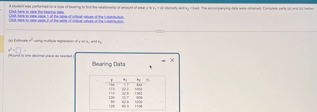
A student was performed on a type of bearing to find the relationship of amount of wear y to x, oil viscosity and x2 = load. The accompanying data were obtained. Complete parts (a) and (b) below. Click here to view the bearing data. Click here to view page 1 of the table of critical values of the t-distribution. Click here to view page 2 of the table of critical values of the I-distribution. (a) Estimate o2 using multiple regression of y on x, and x2. (Round to one decimal place as needed.) Bearing Data y X1 X2 194 1.7 844 173 22.2 1052 114 32.9 1362 230 15.7 809 95 42.9 1205 128 40.3 1106 - X

The average life expectancy of tires 40,000 miles. The company has rece The manager hopes to find out wheth life test, 40 tires were used, and their following SPSS results: One-Sample Statistics Std. Dev Mean time 40881.8262 40 2945 One- df Sig. (2-taile 1.893 Set up Ho: M = 40,000 %3D HA: The test statistic is 1.893 The distribution of the test stati Make the statistical decision (o Express the statistical decision

No tortilla chip aficionado likes soggy chips, so it is important to find characteristics of the production process that produce chips with an appealing texture. The following data on x = frying time (sec) and y = moisture content (%) appeared in an article. x 5 10 15 20 25 30 45 60 y 16.4 9.7 8.1 4.2 3.3 2.8 2.0 1.2 (a) Construct a scatter plot of y versus x. y 15 10- 5 y 15 O 10 10 20 30 40 50 5 10 20 10 NE X 50 60 30 60 40 X 15 y 10 O 5 O y 15 10 20 30 40 50 60 10 20 30 Comment. The plot has a curved pattern. A linear model would not be appropriate. O The plot has a curved pattern. A linear model would be appropriate. O The plot does not have a curved pattern. A linear model would be appropriate. O The plot does not have a curved pattern. A linear model would not be appropriate. 40 50 60 X X

Cathy makes a single deposit into an account earning 2.5% compounded monthly. After five years the account contains $3057.46.how much did she deposit?

Refer to the accompanying data display that results from a sample of airport data speeds in Mbps. Complete parts (a) through (c) below. TInterval (13.046,22.15) x= 17,598 Sx = 16.01712719 E Click the icon to view at distribution table. n= 50 a. What is the number of degrees of freedom that should be used for finding the critical value t,,/2? df =D (Type a whole number.) b. Find the critical value t,/2 corresponding to a 95% confidence level. ta/2 =0 (Round to two decimal places as needed.) c. Give a brief general description of the number of degrees of freedom. O A. The number of degrees of freedom for a collection of sample data is the number of sample values that are determined after certain restrictions have been imposed on all data values. O B. The number of degrees of freedom for a collection of sample data is the total number of sample values. O C. The number of degrees of freedom for a collection of sample data is the number of sample values that can vary after certain…

Wrinkle recovery angle and tensile strength are the two most important characteristics for evaluating the performance of crosslinked cotton fabric. An increase in the degree of crosslinking, as determined by ester carboxyl band absorbance, improves the wrinkle resistance of the fabric (at the expense of reducing mechanical strength). The accompanying data on x = absorbance and y = wrinkle resistance angle was read from a graph in the paper "Predicting the Performance of Durable Press Finished Cotton Fabric with Infrared Spectroscopy".† x 0.115 0.126 0.183 0.246 0.282 0.344 0.355 0.452 0.491 0.554 0.651 y 334 342 355 363 365 372 381 392 400 412 420 Here is regression output from Minitab: Predictor Constant absorb S = 3.60498 Coef 321.878 156.711 SOURCE Regression Residual Error Total SE Coef 2.483 6.464 R-Sq = 98.5% DF 1 9 10 SS 7639.0 117.0 7756.0 T 129.64 24.24 0.000 0.000 R-Sq (adj) = 98.3% MS 7639.0 13.0 F P 587.81 (a) Does the simple linear regression model appear to be…

Laetisaric acid is a compound that holds promise for control of fungus diseases in crop plants. The accompanying data show the results of growing the fungus Pythium (y) in various concentrations of laetisaric acid (x). Laetisaric acid concentration (uG/mL) Fungus growth (mm) 0. 33.3 31.0 29.8 27.8 6. 28.0 6. 29.0 10 25.5 10 23.8 20 18.3 20 15.5 30 11.7 30 10.0 Mean 11.500 23.642 Standard deviation 10.884 7.8471 T =-0.98754 %3D a. State the linear regression equation, and with a 0.01 level of significance, predict the amount (in mm) of fungus growth when 25 uG/mL laetisaric acid is applied. Assume the pairs of data follow a bivariate normal distribution and that the scatterplot shows no evidence of a non-linear relationship in the data. b. Determine the percentage of the variation in fungus growth that is explained by the linear relationship between laetisaric acid concentration and fungus growth. Attack Eil

Water is poured into a large, cone-shaped cistern. The volume of water, measured in cm, is reported at Which of the following would linearize the data for volume and time? different time intervals, measured in seconds. The scatterplot of volume versus time showed a curved Seconds, cm3 O In(Seconds), cm3 Seconds, In(cm') pattern. O In(Seconds), In(cm³)

PLEASE ANSWER ALL THE PARTS OF QUESTION (THIS IS NOT A HRADED ASSIGNMENT)

B6. Pinan Insurance Company wants to study the relationship between the amount of fire damage and the distance between the burning house and the nearest fire station. This information will be used in setting rates for insurance coverage. For a sample of 30 claims for the last year, the director of the actuarial department determined the distance from the fire station (x) and the amount of fire damage, in thousands of dollars (y). The MegaStat output is reported below. ANOVA table Source Regression Residual Total Regression output Variables Intercept Distance-X Answer the following questions. SS 1,864.5782 1,344.4934 3,209.07 Coefficients 12.3601 4.7956 df 1 28 29 MS 1,864.5782 48.0176 Std. Error 3.2915 0.7696 F 38.83 t(df=28) 3.755 6.231 a) Write out the regression equation. Is there a direct or indirect relationship between the distance from the fire station and the amount of fire damage? b) How much damage would you estimate for a fire 5 miles from the nearest fire station?