MATLAB: An Introduction with Applications
6th Edition
ISBN: 9781119256830
Author: Amos Gilat
Publisher: John Wiley & Sons Inc
expand_more
expand_more
format_list_bulleted
Question
![Suppose that a recent poll found that 60% of adults believe that the overall state of moral values is poor. Complete parts (a) through (c).
(a) For 400 randomly selected adults, compute the mean and standard deviation of the random variable X, the number of adults who believe that the overall state of moral values is poor.
The mean of X is 240. (Round to the nearest whole number as needed.)
The standard deviation of X is [blank]. (Round to the nearest tenth as needed.)](https://content.bartleby.com/qna-images/question/ac3be618-b645-4bd8-855b-808ff3fc18d4/e62052d6-b29e-496b-bc86-e97a92a27bff/h6s7j4_thumbnail.png)
Transcribed Image Text:Suppose that a recent poll found that 60% of adults believe that the overall state of moral values is poor. Complete parts (a) through (c).
(a) For 400 randomly selected adults, compute the mean and standard deviation of the random variable X, the number of adults who believe that the overall state of moral values is poor.
The mean of X is 240. (Round to the nearest whole number as needed.)
The standard deviation of X is [blank]. (Round to the nearest tenth as needed.)
Expert Solution
This question has been solved!
Explore an expertly crafted, step-by-step solution for a thorough understanding of key concepts.
This is a popular solution
Trending nowThis is a popular solution!
Step by stepSolved in 3 steps

Follow-up Questions
Read through expert solutions to related follow-up questions below.
Follow-up Question

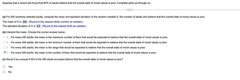
Transcribed Image Text:Suppose that a recent poll found that 60% of adults believe that the overall state of moral values is poor. Complete parts (a) through (c).
(a) For 400 randomly selected adults, compute the mean and standard deviation of the random variable X, the number of adults who believe that the overall state of moral values is poor.
The mean of X is 240. (Round to the nearest whole number as needed.)
The standard deviation of X is 9.8. (Round to the nearest tenth as needed.)
(b) Interpret the mean. Choose the correct answer below.
A. For every 240 adults, the mean is the maximum number of them that would be expected to believe that the overall state of moral values is poor.
B. For every 400 adults, the mean is the minimum number of them that would be expected to believe that the overall state of moral values is poor.
C. For every 400 adults, the mean is the range that would be expected to believe that the overall state of moral values is poor.
D. For every 400 adults, the mean is the number of them that would be expected to believe that the overall state of moral values is poor.
(c) Would it be unusual if 233 of the 400 adults surveyed believe that the overall state of moral values is poor?
Yes
No
Solution
by Bartleby Expert
Follow-up Question

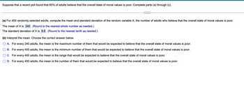
Transcribed Image Text:Suppose that a recent poll found that 60% of adults believe that the overall state of moral values is poor. Complete parts (a) through (c).
(a) For 400 randomly selected adults, compute the mean and standard deviation of the random variable X, the number of adults who believe that the overall state of moral values is poor.
The mean of X is 240. (Round to the nearest whole number as needed.)
The standard deviation of X is 9.8. (Round to the nearest tenth as needed.)
(b) Interpret the mean. Choose the correct answer below.
A. For every 240 adults, the mean is the maximum number of them that would be expected to believe that the overall state of moral values is poor.
B. For every 400 adults, the mean is the minimum number of them that would be expected to believe that the overall state of moral values is poor.
C. For every 400 adults, the mean is the range that would be expected to believe that the overall state of moral values is poor.
D. For every 400 adults, the mean is the number of them that would be expected to believe that the overall state of moral values is poor.
Solution
by Bartleby Expert
Follow-up Questions
Read through expert solutions to related follow-up questions below.
Follow-up Question

Transcribed Image Text:Suppose that a recent poll found that 60% of adults believe that the overall state of moral values is poor. Complete parts (a) through (c).
(a) For 400 randomly selected adults, compute the mean and standard deviation of the random variable X, the number of adults who believe that the overall state of moral values is poor.
The mean of X is 240. (Round to the nearest whole number as needed.)
The standard deviation of X is 9.8. (Round to the nearest tenth as needed.)
(b) Interpret the mean. Choose the correct answer below.
A. For every 240 adults, the mean is the maximum number of them that would be expected to believe that the overall state of moral values is poor.
B. For every 400 adults, the mean is the minimum number of them that would be expected to believe that the overall state of moral values is poor.
C. For every 400 adults, the mean is the range that would be expected to believe that the overall state of moral values is poor.
D. For every 400 adults, the mean is the number of them that would be expected to believe that the overall state of moral values is poor.
(c) Would it be unusual if 233 of the 400 adults surveyed believe that the overall state of moral values is poor?
Yes
No
Solution
by Bartleby Expert
Follow-up Question

Transcribed Image Text:Suppose that a recent poll found that 60% of adults believe that the overall state of moral values is poor. Complete parts (a) through (c).
(a) For 400 randomly selected adults, compute the mean and standard deviation of the random variable X, the number of adults who believe that the overall state of moral values is poor.
The mean of X is 240. (Round to the nearest whole number as needed.)
The standard deviation of X is 9.8. (Round to the nearest tenth as needed.)
(b) Interpret the mean. Choose the correct answer below.
A. For every 240 adults, the mean is the maximum number of them that would be expected to believe that the overall state of moral values is poor.
B. For every 400 adults, the mean is the minimum number of them that would be expected to believe that the overall state of moral values is poor.
C. For every 400 adults, the mean is the range that would be expected to believe that the overall state of moral values is poor.
D. For every 400 adults, the mean is the number of them that would be expected to believe that the overall state of moral values is poor.
Solution
by Bartleby Expert
Knowledge Booster
Similar questions
- In preparation for the upcoming school year, a teacher looks at raw test scores on the statewide standardized test for the students in her class. Instead of looking at the scores relative to the norms in the state, the teacher wants to understand the scores relative to the students who will be in the class. To do so, she decides to convert the test scores into z-scores relative to the mean and standard deviation of the students in the class. The mean test score in her upcoming class is 49, and the standard deviation is 20.7. The teacher now wants to identify those students who may need extra help. She decides to look at students who have z-scores below z = -2.00 Identify the test score corresponding to a z-score of below z = -2.00. Round to the nearest whole number.arrow_forwardSuppose the scores of students on an exam are Normally distributed with a mean of 522 and a standard deviation of 83. Then approximately 99.7% of the exam scores lie between the numbers such that the mean is halfway between these two integers. and ☐arrow_forwardThe following table shows the number of people that have either 0, 1, 2 or 3 cars registered in their name, from a sample of 311 people. x n 0 93 1 91 2 60 3 67 (a) Find the mean number of cars owned for this sample. Give your answer to at least 2 decimal places. (b) Find the standard deviation of cars owned for this sample. Give your answer to at least 2 decimal places.arrow_forward
- Use z scores to compare the given values. The tallest living man at one time had a height of 238 cm. The shortest living man at that time had a height of 142.4 cm. Heights of men at that time had a mean of 175.45 cm and a standard deviation of 5.59 cm. Which of these two men had the height that was more extreme? ... Since the z score for the tallest man is z = 0 and the z score for the shortest man is z = the man had the height that was Im- more extreme. (Round to two decimal places.) shortest tallestarrow_forwardn a school district, all sixth grade students take the same standardized test. The superintendant of the school district takes a random sample of 21 scores from all of the students who took the test. She sees that the mean score is 128 with a standard deviation of 41.4416. The superintendant wants to know if the standard deviation has changed this year. Previously, the population standard deviation was 25. Is there evidence that the standard deviation of test scores has increased at the α=0.005 level? Assume the population is normally distributed. Step 1 of 5 : State the null and alternative hypotheses. Round to four decimal places when necessary.arrow_forwardChebyshev's Theorem states that for any distribution of numerical data, at least 1-1/k? of the numbers lie within The percent of numbers between 88 and 112 is at least %. k standard deviations of the mean. (Round to the nearest hundredth as needed.) In a certain distribution of numbers, the mean is 100, with a standard deviation of 6. Use Chebyshev's Theorem to tell what percent of the numbers are between 88 and 112.arrow_forward
- For college-bound seniors in 2018, SAT math scores are normally distributed with a mean of 515 and a standard deviation of 116. You suspect that seniors in the Auraria Campus are much brighter than the country as a whole, so you decide to conduct a test. In a random sample of 25 seniors, you find the mean SAT math score to be 555. You assume that the standard deviation of math scores in Auraria Campus are the same as the national standard deviation of a = 116. Is this sufficient evidence to conclude that Auraria Campus seniors are smarter? Take a -0.05.arrow_forwardOn an intelligence test, the mean number of raw items correct is 236 and the standard deviation is 39. What are the raw (actual) scores on the test for people with IQs of (a) 119, (b) 81, and (c)100? To do this problem, first figure the Z score for the particular IQ score; then use that Z score to find the raw score. Note that IQ scores have a mean of 100 and a standard deviation of 15. (a) What is the raw (actual) score on the test for people with an IQ of 119?arrow_forwardA standardized exam's scores are normally distributed. In a recent year, the mean test score was 1458 and the standard deviation was 312. The test scores of four students selected at random are 1860, 1220, 2150, and 1340. Find the z-scores that correspond to each value and determine whether any of the values are unusual. The z-score for 1860 is (Round to two decimal plaes as needed.)arrow_forward
- A professor believes that, for the introductory art history classes at his university, the mean test score of students in the evening classes is lower than the mean test score of students in the morning classes. He collects data from a random sample of 250 students in evening classes and finds that they have a mean test score of 85.6. He knows the population standard deviation for the evening classes to be 4.6 points. A random sample of 150 students from morning classes results in a mean test score of 86.7. He knows the population standard deviation for the morning classes to be 8.3 points. Test his claim with a 99 % level of confidence. Let students in the evening classes be Population 1 and let students in the morning classes be Population 2. Step 3 of 3: Draw a conclusion and interpret the decision. Answer 围 Tables E Keypad Keyboard Shortcuts We fail to reject the null hypothesis and conclude that there is sufficient evidence at a 0.01 level of significance to support the…arrow_forwardThe salaries of professional baseball players are heavily skewed right with a mean of $3.2 million and a standard deviation of $2 million. The salaries of professional football players are also heavily skewed right with a mean of $1.9 million and a standard deviation of $1.5 million. A random sample of 40 baseball players’ salaries and 35 football players’ salaries is selected. The mean salary is determined for both samples. Let represent the difference in the mean salaries for baseball and football players. Which of the following represents the shape of the sampling distribution for ? skewed right since the populations are both right skewed skewed right since the differences in salaries cannot be negative approximately Normal since both sample sizes are greater than 30 approximately Normal since the sum of the sample sizes is greater than 30arrow_forward
arrow_back_ios
arrow_forward_ios
Recommended textbooks for you
 MATLAB: An Introduction with ApplicationsStatisticsISBN:9781119256830Author:Amos GilatPublisher:John Wiley & Sons Inc
 Probability and Statistics for Engineering and th...StatisticsISBN:9781305251809Author:Jay L. DevorePublisher:Cengage Learning
 Statistics for The Behavioral Sciences (MindTap C...StatisticsISBN:9781305504912Author:Frederick J Gravetter, Larry B. WallnauPublisher:Cengage Learning
 Elementary Statistics: Picturing the World (7th E...StatisticsISBN:9780134683416Author:Ron Larson, Betsy FarberPublisher:PEARSON
 The Basic Practice of StatisticsStatisticsISBN:9781319042578Author:David S. Moore, William I. Notz, Michael A. FlignerPublisher:W. H. Freeman
 Introduction to the Practice of StatisticsStatisticsISBN:9781319013387Author:David S. Moore, George P. McCabe, Bruce A. CraigPublisher:W. H. Freeman

MATLAB: An Introduction with Applications
Statistics
ISBN:9781119256830
Author:Amos Gilat
Publisher:John Wiley & Sons Inc

Probability and Statistics for Engineering and th...
Statistics
ISBN:9781305251809
Author:Jay L. Devore
Publisher:Cengage Learning

Statistics for The Behavioral Sciences (MindTap C...
Statistics
ISBN:9781305504912
Author:Frederick J Gravetter, Larry B. Wallnau
Publisher:Cengage Learning

Elementary Statistics: Picturing the World (7th E...
Statistics
ISBN:9780134683416
Author:Ron Larson, Betsy Farber
Publisher:PEARSON

The Basic Practice of Statistics
Statistics
ISBN:9781319042578
Author:David S. Moore, William I. Notz, Michael A. Fligner
Publisher:W. H. Freeman

Introduction to the Practice of Statistics
Statistics
ISBN:9781319013387
Author:David S. Moore, George P. McCabe, Bruce A. Craig
Publisher:W. H. Freeman