
MATLAB: An Introduction with Applications
6th Edition
ISBN: 9781119256830
Author: Amos Gilat
Publisher: John Wiley & Sons Inc
expand_more
expand_more
format_list_bulleted
Related questions
Question
Square this value (r2). Include the value and describe this
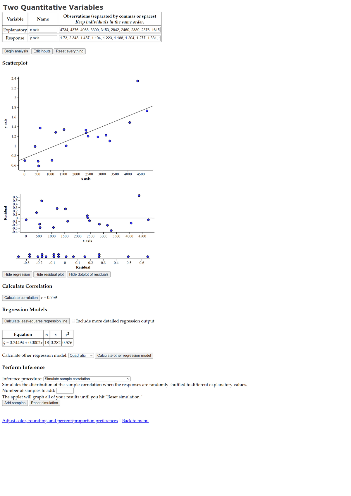

Transcribed Image Text:Two Quantitative Variables
Variable
Explanatory|x axis
Response y axis
Begin analysis Edit inputs
Scatterplot
y axis
Residual
2.4-
2.2.
2-
1.8
1.6-
1.4-
1.2-
1
0.8
0.6-
0.6
0.5
0.4
0.3
0.2
0.1
0
-0.1
-0.2
-0.3
-0.4
O
Name
0
0
•
OO
500 1000 1500 2000 2500 3000 3500 4000 4500
x axis
O
500 1000 1500
-0.3 -0.2 -0.1
Calculate Correlation
Observations (separated by commas or spaces)
Keep individuals in the same order.
4734, 4376, 4068, 3300, 3153, 2842, 2460, 2389, 2376, 1615
1.73, 2.348, 1.487, 1.104, 1.223, 1.188, 1.204, 1.277, 1.331, |
Reset everything
Hide regression Hide residual plot
Calculate correlation r=0.759
Regression Models
T
0
n
Calculate least-squares regression line
Equation
= 0.74494 + 0.0002x 18 0.282 0.576
S²
2000 2500 3000 3500 4000 4500
x axis
0.1
Residual
Hide dotplot of residuals
0.2
0.3
Calculate other regression model: [Quadratic
Perform Inference
0.4
0.5
0.6
Include more detailed regression output
Calculate other regression model
Inference procedure: [Simulate sample correlation
Simulates the distribution of the sample correlation when the responses are randomly shuffled to different explanatory values.
Number of samples to add: |
The applet will graph all of your results until you hit "Reset simulation."
Add samples
Reset simulation
Adjust color, rounding, and percent/proportion preferences | Back to menu
Expert Solution
This question has been solved!
Explore an expertly crafted, step-by-step solution for a thorough understanding of key concepts.

Step by stepSolved in 3 steps

Knowledge Booster

Similar questions
- Which correlation would allows for the best prediction of Y based on X? Group of answer choices r = .50 r = .80 r = .05 r = -.90arrow_forwardAnswer clearlyarrow_forwardUse the table to find the following, unit price being your (x) and units sold (y). a. Find linear correlation coefficient. Years of Experience Salary in 1000$ 2 3. 15 28 42 13 64 50 16 90 11 58 8 54 b. Find the line of best fit. c. How many units will sell if the unit price was 0.85.arrow_forward
- Briefly explain the difference between leading, coincident, and lagging indicators.arrow_forwardCorrelation does not imply causation. What does this mean? Find an example in the media that needs to understand this concept and explain it to your peers. Be sure to include the link to the example you are using.arrow_forwardThe more serving of fruits and vegetables that people tend to eat during the week, the lower their levels of cholesterol. What type of correlation vegetables eaten and cholesterol levels? A positive B negativearrow_forward
- Construct a scatter plot from the given points and describe the correlation.arrow_forwardGive an example of two variables that you would expect to have a correlation close to or equal to -1. Give an example of two variables that you would expect to have a correlation close to or equal to 0. Remember that survey question you wrote? Take the class responses to your survey as data related to the one variable of your question. Now, take the list of responses from the survey question that one of your classmates wrote. Write down both lists of data. (If one sample size happens to be different from the other, cut the larger sample size down to that of the smaller sample size.) Calculate the correlation between the two variables. Describe the linear relationship between these two variables. (data for number 3) How many cars have you had so far in your lifetime? 0,1,1,1,2,2,2,2,3,3,3,3,4,4,5,6,6,7,10. How many days per week do you exercise? 0,0,0,1,2,3,3,3,3,4,4,4,4,5,5,5,5,6,6,6arrow_forwardSolve.arrow_forward
- The table shows total earnings, y (in dollars ), of a food x,0,1,2,3,4,5,6 y,0,18,40,62,77,85,113 a. Make a scatter plot. b. What type of correlation is shown in the graarrow_forwardCompute and interpret the coefficient of multiple correlation. Number 4 answer is missing.arrow_forwardr = - 1arrow_forward
arrow_back_ios
arrow_forward_ios
Recommended textbooks for you
- MATLAB: An Introduction with ApplicationsStatisticsISBN:9781119256830Author:Amos GilatPublisher:John Wiley & Sons Inc
 Probability and Statistics for Engineering and th...StatisticsISBN:9781305251809Author:Jay L. DevorePublisher:Cengage Learning
 Statistics for The Behavioral Sciences (MindTap C...StatisticsISBN:9781305504912Author:Frederick J Gravetter, Larry B. WallnauPublisher:Cengage Learning
  Elementary Statistics: Picturing the World (7th E...StatisticsISBN:9780134683416Author:Ron Larson, Betsy FarberPublisher:PEARSON
 The Basic Practice of StatisticsStatisticsISBN:9781319042578Author:David S. Moore, William I. Notz, Michael A. FlignerPublisher:W. H. Freeman
 Introduction to the Practice of StatisticsStatisticsISBN:9781319013387Author:David S. Moore, George P. McCabe, Bruce A. CraigPublisher:W. H. Freeman
MATLAB: An Introduction with Applications
Statistics
ISBN:9781119256830
Author:Amos Gilat
Publisher:John Wiley & Sons Inc
Probability and Statistics for Engineering and th...
Statistics
ISBN:9781305251809
Author:Jay L. Devore
Publisher:Cengage Learning
Statistics for The Behavioral Sciences (MindTap C...
Statistics
ISBN:9781305504912
Author:Frederick J Gravetter, Larry B. Wallnau
Publisher:Cengage Learning
Elementary Statistics: Picturing the World (7th E...
Statistics
ISBN:9780134683416
Author:Ron Larson, Betsy Farber
Publisher:PEARSON
The Basic Practice of Statistics
Statistics
ISBN:9781319042578
Author:David S. Moore, William I. Notz, Michael A. Fligner
Publisher:W. H. Freeman
Introduction to the Practice of Statistics
Statistics
ISBN:9781319013387
Author:David S. Moore, George P. McCabe, Bruce A. Craig
Publisher:W. H. Freeman