
MATLAB: An Introduction with Applications
6th Edition
ISBN: 9781119256830
Author: Amos Gilat
Publisher: John Wiley & Sons Inc
expand_more
expand_more
format_list_bulleted
Related questions
Concept explainers
Question
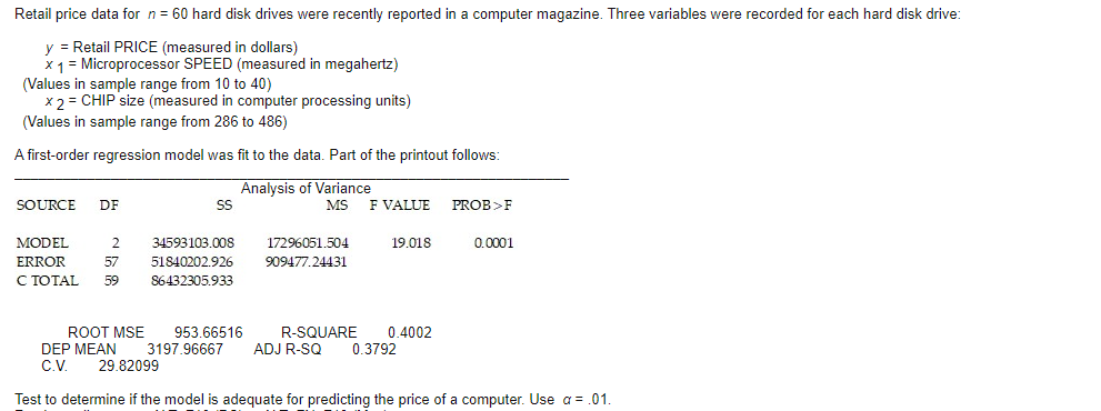

Transcribed Image Text:Retail price data for n = 60 hard disk drives were recently reported in a computer magazine. Three variables were recorded for each hard disk drive:
y = Retail PRICE (measured in dollars)
x1= Microprocessor SPEED (measured in megahertz)
(Values in sample range from 10 to 40)
x2 = CHIP size (measured in computer processing units)
(Values in sample range from 286 to 486)
A first-order regression model was fit to the data. Part of the printout follows:
Analysis of Variance
SOURCE
DF
MS
F VALUE
PROB>F
MODEL
2
34593103.008
17296051,504
19.018
0.0001
ERROR
57
51840202.926
909477.24431
C TOTAL
59
86432305.933
ROOT MSE
953.66516
3197.96667
R-SQUARE
0.4002
0.3792
DEP MEAN
CV.
ADJ R-SQ
29.82099
Test to determine if the model is adequate for predicting the price of a computer. Use a = .01.
Expert Solution
This question has been solved!
Explore an expertly crafted, step-by-step solution for a thorough understanding of key concepts.

This is a popular solution

Trending nowThis is a popular solution!

Step by stepSolved in 2 steps

Knowledge Booster


Learn more about
Need a deep-dive on the concept behind this application? Look no further. Learn more about this topic, statistics and related others by exploring similar questions and additional content below.Similar questions
- The table below gives the age and bone density for five randomly selected women. Using this data, consider the equation of the regression line, yˆ=b0+b1x, for predicting a woman's bone density based on her age. Keep in mind, the correlation coefficient may or may not be statistically significant for the data given. Remember, in practice, it would not be appropriate to use the regression line to make a prediction if the correlation coefficient is not statistically significant. Age 47 48 56 60 67 Bone Density 359 350 334 314 313 Find the estimated slope. Round your answer to three decimal places.arrow_forwardRetail price data for n = 60 hard disk drives were recently reported in a computer magazine. Three variables were recorded for each hard disk drive: y = Retail PRICE (measured in dollars) X1 = Microprocessor SPEED (measured in megahertz) (Values in sample range from 10 to 40) x 2 = CHIP size (measured in computer processing units) (Values in sample range from 286 to 486) A first-order regression model. was fit to the data. Part of the printout follows: Parameter Estimates T FOR 0 ERROR PARAMETER = 0 PROB>ITI PARAMETER STANDARD VARIABLE DF ESTIMATE INTERCEPT 1 -373.526392 1258.1243396 -0.297 0.7676 SPEED 1 104.838940 22.36298195 4 688 0.0001 сHP 1 3.571850 3.89422935 0.917 0.3629 Identify and interpret the estimate of B2-arrow_forwardA regression model to predict Y, the state burglary rate per 100,000 people, used the following four state predictors: X1 = median age, X2 = number of bankruptcies per 1,000 population, X3 = federal expenditures per capita (a leading predictor), and X4 = high school graduation percentage. Click here for the Excel Data File (a) Using the sample size of 45 people, calculate the tcalc and p-value in the table given below. (Negative values should be indicated by a minus sign. Leave no cells blank - be certain to enter "0" wherever required. Round your t-values to 3 decimal places and p- values to 4 decimal places.) Predictor Intercept AgeMed Coefficient SE tcalc p-value 4,641.0430 798.0634 -28.8630 12.4684 Bankrupt 20.1604 12.1079 FedSpend HSGrad% -0.0181 0.0181 -30.3196 7.1136 (b-1) What is the critical value of Student's tin Appendix D for a two-tailed test at a = .01? (Round your answer to 3 decimal places.) -value =arrow_forward
- The local utility company surveys 12 randomly selected customers. For each survey participant, the company collects the following: annual electric bill (in dollars) and home size (in square feet). Output from a regression analysis appears below: Bill = 15.9 + 4.45*Size Coefficients Estimate Std. Error (Intercept) 15.9 0.3 Size 4.45 0.57 We are 98% confident that the mean annual electric bill increases by between dollars and dollars for every additional square foot in home size.arrow_forwardSuppose the estimaited OLS regression is: Happiness = a + b*dailychocolates Now use chocolate consumprion per week instead of days. What is the relationship between the old and new units? How would this affect b (i.e. what is bnew in terms of b)?arrow_forwardThe local utility company surveys 12 randomly selected customers. For each survey participant, the company collects the following: annual electric bill (in dollars) and home size (in square feet). Output from a regression analysis is as follows: bill = 16.2 + 3.58. size. Coefficients Estimate Std. Error (Intercept) 16.2 Size 3.58 0.47 0.68 Round your answer to three decimal places, and round any interim calculations to four decimal places. We are 99% confident that the mean annual electric bill increases by between dollars for every additional square foot in home size. dollars andarrow_forward
- For Data Set 9 in Appendix B, “Bear Measurements,” we get this regression equation: Weight = -274 + 0.426 Length + 12.1 Chest Size, with R2 = 0.928. Interpret the multiple coefficient of determination – what does this value tell us?arrow_forwardThe table below gives the age and bone density for five randomly selected women. Using this data, consider the equation of the regression line, y = bo + bjx, for predicting a woman's bone density based on her age. Keep in mind, the correlation coefficient may or may not be statistically significant for the data given. Remember, in practice, it would not be appropriate to use the regression line to make a prediction if the correlation coefficient is not statistically significant. Age 47 49 50 51 58 Bone Density 360 353 336 333 310 Table Copy Data Step 1 of 6: Find the estimated slope. Round your answer to three decimal places.arrow_forwardThe table below gives the number of weeks of gestation and the birth weight (in pounds) for a sample of five randomly selected babies. Using this data, consider the equation of the regression line, y based on the number of weeks of gestation. Keep in mind, the correlation coefficient may or may not be statistically significant for the data given. Remember, in practice, it would not be appropriate to use the regression line to make a prediction if the correlation coefficient is not statistically significant. bo + bjx, for predicting the birth weight of a baby Weeks of Gestation 33 35 37 39 40 Weight (in pounds) 5 6.8 7.9 8.5 9.3 Table Copy Data Step 5 of 6: Find the error prediction when x = 39. Round your answer to three decimal places.arrow_forward
- The table below gives the age and bone density for five randomly selected women. Using this data, consider the equation of the regression line, yˆ=b0+b1x, for predicting a woman's bone density based on her age. Keep in mind, the correlation coefficient may or may not be statistically significant for the data given. Remember, in practice, it would not be appropriate to use the regression line to make a prediction if the correlation coefficient is not statistically significant. Age Bone Density48 35151 32056 31860 31169 310 Step 6 of 6: Find the value of the coefficient of determination. Round your answer to three decimal places.arrow_forwardThe table below gives the age and bone density for five randomly selected women. Using this data, consider the equation of the regression line, yˆ=b0+b1x, for predicting a woman's bone density based on her age. Keep in mind, the correlation coefficient may or may not be statistically significant for the data given. Remember, in practice, it would not be appropriate to use the regression line to make a prediction if the correlation coefficient is not statistically significant. Age 35 43 53 54 55 Bone Density 350 340 339 321 310 Table Step 6 of 6 : Find the value of the coefficient of determination. Round your answerarrow_forwardThe datasetBody.xlsgives the percent of weight made up of body fat for 100 men as well as other variables such as Age, Weight (lb), Height (in), and circumference (cm) measurements for the Neck, Chest, Abdomen, Ankle, Biceps, and Wrist. We are interested in predicting body fat based on abdomen circumference. Find the equation of the regression line relating to body fat and abdomen circumference. Make a scatter-plot with a regression line. What body fat percent does the line predict for a person with an abdomen circumference of 110 cm? One of the men in the study had an abdomen circumference of 92.4 cm and a body fat of 22.5 percent. Find the residual that corresponds to this observation. Bodyfat Abdomen 32.3 115.6 22.5 92.4 22 86 12.3 85.2 20.5 95.6 22.6 100 28.7 103.1 21.3 89.6 29.9 110.3 21.3 100.5 29.9 100.5 20.4 98.9 16.9 90.3 14.7 83.3 10.8 73.7 26.7 94.9 11.3 86.7 18.1 87.5 8.8 82.8 11.8 83.3 11 83.6 14.9 87 31.9 108.5 17.3…arrow_forward
arrow_back_ios
SEE MORE QUESTIONS
arrow_forward_ios
Recommended textbooks for you
- MATLAB: An Introduction with ApplicationsStatisticsISBN:9781119256830Author:Amos GilatPublisher:John Wiley & Sons Inc
 Probability and Statistics for Engineering and th...StatisticsISBN:9781305251809Author:Jay L. DevorePublisher:Cengage Learning
 Statistics for The Behavioral Sciences (MindTap C...StatisticsISBN:9781305504912Author:Frederick J Gravetter, Larry B. WallnauPublisher:Cengage Learning
  Elementary Statistics: Picturing the World (7th E...StatisticsISBN:9780134683416Author:Ron Larson, Betsy FarberPublisher:PEARSON
 The Basic Practice of StatisticsStatisticsISBN:9781319042578Author:David S. Moore, William I. Notz, Michael A. FlignerPublisher:W. H. Freeman
 Introduction to the Practice of StatisticsStatisticsISBN:9781319013387Author:David S. Moore, George P. McCabe, Bruce A. CraigPublisher:W. H. Freeman
MATLAB: An Introduction with Applications
Statistics
ISBN:9781119256830
Author:Amos Gilat
Publisher:John Wiley & Sons Inc
Probability and Statistics for Engineering and th...
Statistics
ISBN:9781305251809
Author:Jay L. Devore
Publisher:Cengage Learning
Statistics for The Behavioral Sciences (MindTap C...
Statistics
ISBN:9781305504912
Author:Frederick J Gravetter, Larry B. Wallnau
Publisher:Cengage Learning
Elementary Statistics: Picturing the World (7th E...
Statistics
ISBN:9780134683416
Author:Ron Larson, Betsy Farber
Publisher:PEARSON
The Basic Practice of Statistics
Statistics
ISBN:9781319042578
Author:David S. Moore, William I. Notz, Michael A. Fligner
Publisher:W. H. Freeman
Introduction to the Practice of Statistics
Statistics
ISBN:9781319013387
Author:David S. Moore, George P. McCabe, Bruce A. Craig
Publisher:W. H. Freeman