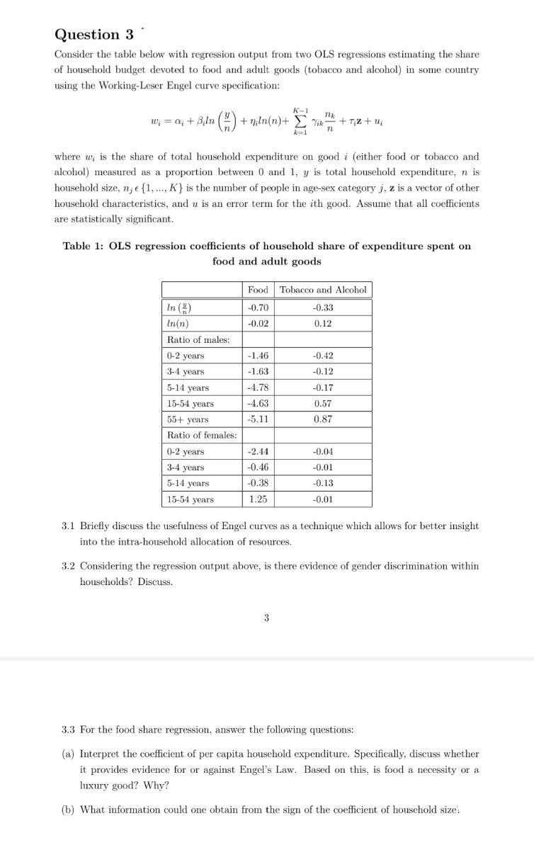
Question 3 Consider the table below with regression output from two OLS regressions estimating the share of household budget devoted to food and adult goods (tobacco and alcohol) in some country using the Working-Leser Engel curve specification: K-1 Thk w₁ = a₁ + Bln (²) + nin(n) + Σ Tik +7₁2+U₂ n k=1 where w, is the share of total household expenditure on good i (either food or tobacco and alcohol) measured as a proportion between 0 and 1, y is total household expenditure, n is household size, n, e {1,..., K} is the number of people in age-sex category j, z is a vector of other household characteristics, and u is an error term for the ith good. Assume that all coefficients are statistically significant. Table 1: OLS regression coefficients of household share of expenditure spent on food and adult goods In (2) In(n) Ratio of males: 0-2 years. 3-4 years 5-14 years 15-54 years 55+ years Ratio of females: 0-2 years 3-4 years 5-14 years 15-54 years Food Tobacco and Alcohol -0.70 -0.33 -0.02 0.12 -1.46 -1.63 -4.78 -4.63 -5.11 -2.44 -0.46 -0.38 1.25 -0.42 -0.12 -0.17 0.57 0.87 -0.04 -0.01 -0.13 -0.01 3.1 Briefly discuss the usefulness of Engel curves as a technique which allows for better insight into the intra-household allocation of resources. 3 3.2 Considering the regression output above, is there evidence of gender discrimination within households? Discuss. 3.3 For the food share regression, answer the following questions: (a) Interpret the coefficient of per capita household expenditure. Specifically, discuss whether it provides evidence for or against Engel's Law. Based on this, is food a necessity or a luxury good? Why? (b) What information could one obtain from the sign of the coefficient of household size:

You are interested in how the number of hours a high school student has to work in an outside job has on their GPA. In your regression you want to control for high school standing and so you run the following regression: GPA = 3.4 0.03 * HrsWrk - 0.7 * Frosh - 0.3 * Soph +0.1 * Junior (1.1) (0.013) (0.23) (0.14) (0.08) where HrsWrk is the number of hours the student works per week, and Frosh, Soph, and Junior are dummy variables for the student's class standing. a) If you include a dummy variable for seniors, that would cause a Hint: type one word in each blank. For the rest of questions, type a number in one decimal place. b) The expected GPA of a Sophomore who works 10 hours per week is c) The expected GPA of a Senior who works 10 hours per week is d) If Dom and Sarah work the same number of hours per week, but Dom is a Junior and Sarah is a Freshman. Dom is expected to have a higher GPA than Sarah. e) Suppose you rewrite the regression as: problem. GPA = ₁HrsWrk + ß2Frosh + B2Soph +…

Suppose you run the following regression: outcome=alpha0 + alpha1*female + alpha2*married + epsilon. You know that female equals 1 for females and 0 otherwise. You know that married equals 1 if the person is married and 0 otherwise. What is the estimated outcome for non-married respondents who are not female?

An analyst working for your firm provided an estimated log-linear demand function based on the natural logarithm of the quantity sold, price, and the average income of consumers. Results are summarized in the following table: SUMMARY OUTPUT Regression Statistics Multiple R R Square Adjusted R Square Standard Error Observations ANOVA Regression Residual Total Intercept LN Price LN Income df 0.968 0.937 0.933 0.003 30 SS MS F 2 0.003637484 0.001818742 202.48598 0.000242516 8.98206E-06 27 29 0.00388 Coefficients Standard Error 0.57 0.00 0.13 0.51 -0.08 0.15 t Stat 0.90 -19.50 1.13 P-value 0.37 0.00 0.27 Significance F 5.55598E-17 Lower 95% -0.65 -0.09 -0.12 How would a 4 percent increase in income impact the demand for your product? Demand would increase by 60 percent. Demand would increase by 0.6 percent. Demand would decrease by 60 percent. Demand would decrease by 0.6 percent. Upper 95% 1.68 -0.07 0.41

Using data from a random sample of 1000 working adults, we obtain the following estimated regression to study the effect of experience (exper) on log of wage (log(wage)). log(wage) = 5.423 -0.034ezper +0.009ezper² + 0.082educ + 0.157male What other regression do you need to run to test the null hypothesis that, holding other factors fixed, experience has no effect on log(wage)? Explain what test you would perform.

Your company just became international by offering its products in both the United States and Canada. Experts in your analytics department believe that tastes for your product differ in those two countries, and have carefully collected data on prices and quantity demanded in both countries. They then present you with the results of two regressions, one for each country, as follows: Log Price regressed on Log Quantity (United States): Standard Coefficients Error t Stat P-value Lower 95% Upper 95 % 1.67605E- Intercept 52.75573994 10.81051303 4.88040363 31.48708283 74.0239705 06 | Log Quantity -5.382266173 1.170584108 -4.597932039 6.15253E-06 -7.685279168 -3.079253177 Log Price regressed on Log Quantity (Canada): Standard Error Coefficients 22.8707593 10.64507785 -2.095788278 | 1.152727409 -1.818112644 0.069981782 t Stat 2.148482109 Upper 95% 43.8139384 P-value Lower 95% Intercept Log Quantity 0.032425603 1.9275802 -4.363669916 0.17209336 Assume you have adequate statistical significance…

Consider the following data regarding students' college GPAs and high school GPAs. The estimated regression equation is  Estimated College GPA=1.85+0.4743(High School GPA).Estimated College GPA=1.85+0.4743(High School GPA). GPAs College GPA High School GPA 3.843.84 2.562.56 3.573.57 3.903.90 2.072.07 3.143.14 4.004.00 3.223.22 3.873.87 2.882.88 2.212.21 2.082.08 Copy Data   Step 1 of 3 :   Compute the sum of squared errors (SSE) for the model. Round your answer to four decimal places.

The data for this question is given in the file 1.Q1.xlsx(see image)  and it refers to data for some cities X1 = total overall reported crime rate per 1 million residents X3 = annual police funding in $/resident X7 = % of people 25 years+ with at least 4 years of college   (a) Estimate a regression with X1 as the dependent variable and X3 and X7 as the independent variables. (b) Will additional education help to reduce total overall crime (lead to a statistically significant reduction in crime)? Please explain. (c) Will an increase in funding for the police departments help reduce total overall crime (lead to a statistically significant reduction in total overall crime)? Please explain. (d) If you were asked to recommend a policy to reduce crime, then, based only on the above regression results, would you choose to invest in education (local schools) or in additional funding for the police? Please explain.

Suppose you work for North Dakota DNR Grand Forks office. DNR would like to know whether they should set aside some conservation land, previously slated to be logged, for a potential state park. You are helping do a travel-cost analysis to estimate the benefits of the set-aside. You collected data from 500 visitors who came to a state park in a neighboring state. You ran regression analysis and controlled for these visitors' age, income, education, employment status, and other important factors that might affect the number of visits. With all the information, you have developed the following relationship: (a) (b) Cost to Visit $20 $40 $80 # of Visits Per Person Per Year 8 6 2 Graph the demand curve for the number of visits as a function of the "price" -- the travel cost. Based on demographic information about the people living in the vicinity of the proposed park, you have estimated that 10,000 people will take an average of 4 visits per year. For the average person, calculate: (1) The…

Imagine you are trying to explain the effect of square footage on home sale prices in the United States. You collect a random sample of 100,000 homes that recently sold. a) Homes can be one of three types: single-family houses, townhomes, or condos. How would you control for a home’s type in a regression model? b) Write down a regression model that includes controls for home type, square footage, and number of bedrooms. c) How would you interpret the estimated coefficients for each of the variables from part b? Be specific. Note Don't forget to include dummy variables.