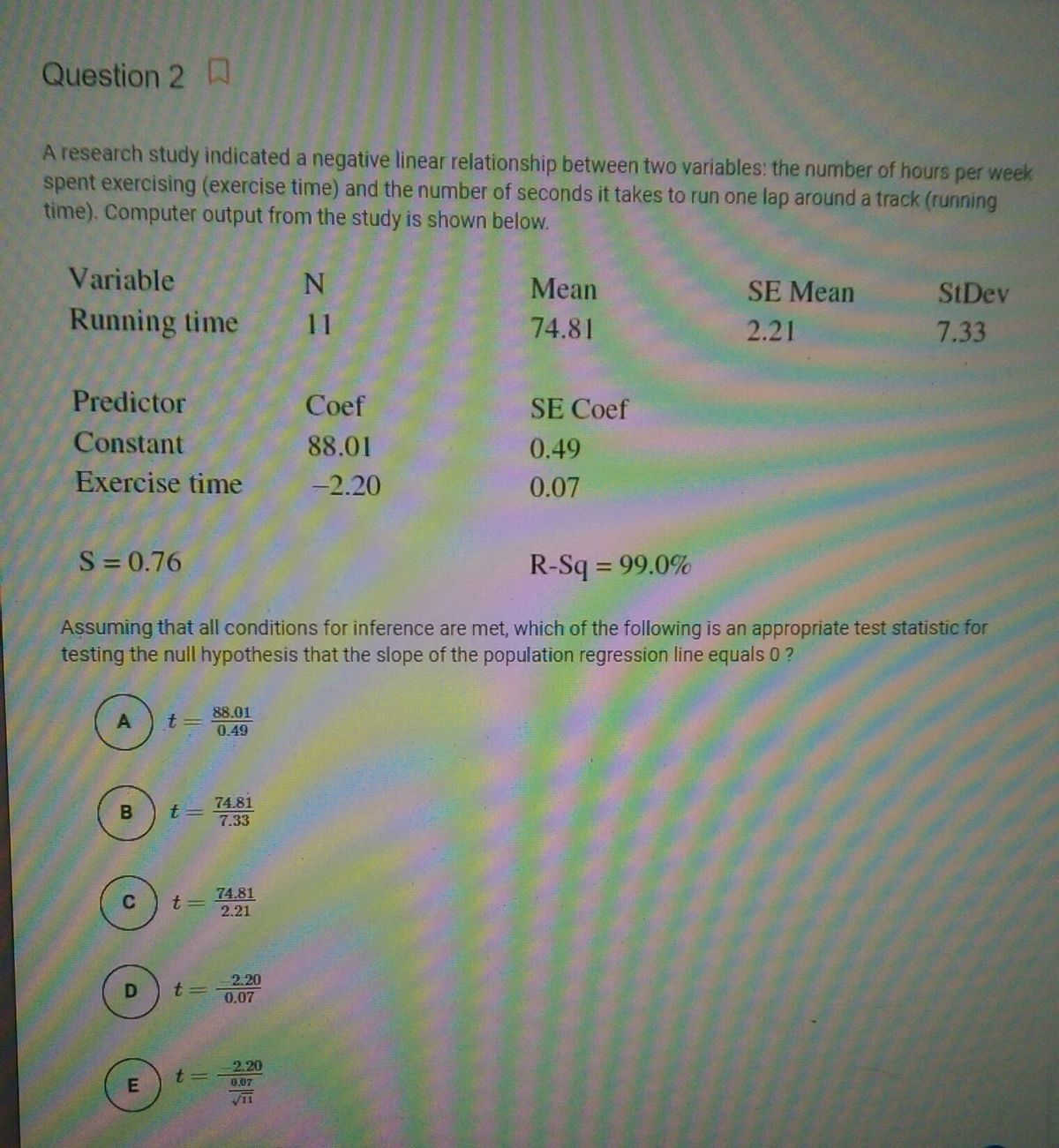
Question 2 A research study indicated a negative linear relationship between two variables: the number of hours spent exercising (exercise time) and the number of seconds it takes to run one lap around a track (running time). Computer output from the study is shown below. per week Variable Mean SE Mean StDev Running time 11 74.81 2.21 7.33 Predictor Coef SE Coef Constant 88.01 0.49 Exercise time -2.20 0.07 S = 0.76 R-Sq = 99.0% %3D Assuming that all conditions for inference are met, which of the following is an appropriate test statistic for testing the null hypothesis that the slope of the population regression line equals 0 ? 88.01 0.49 t = 74.81 7.33 74.81 2.21 t = 2.20 t 3= 0.07 2.20 0.07

PART 3   A car mat manufacture been having quality issues with its production.  A series of tests were carried out to measure the resulting pH of the most common carpet produced, Type 1, as a good indicator of quality. For the following questions show all calculations and formula used.   What is the mean, mode and range of the pH after dyeing? Table – Type 1 pH after addition of dye 5.105 to 5.3 5.305 to 5.5 5.5.05 to 5.7 5.705 to 5.9 5.905 to 6.1 6.105 to 6.3 6.305 to 6.5 No. of samples 1 5 7 8 7 4 1     For pH after addition of dye calculate the standard deviation, showing your calculations in full.   Plot the standard deviation graph in Excel showing the distribution.   From your calculations and the data   Give the minimum and maximum limits the pH may be, given that the distribution is normal. Calculate the probability that a randomly selected carpet sample will have a PH of (i) 6.1 and (ii) 5.4.   Further tests were carried on a…

1. Question 1: The Public Utility Commission is interested in describing the relationship between household monthly utility bills and the size of the house. A recent study of 30 randomly selected household resulted in the following regression results: SUMMARY OUTPUT Regression Statistics Multiple R R Square Adjusted R Square Standard Error 0.149769088 0.02243078 -0.012482407 16.72762259 Observations 30 ANOVA df SS MS 1 179.7725274 179.7725 0.642473 Regression Residual 28 7834.774007 279.8134 Total 29 8014.546534 t Stat 13.44691911 4.941135 3.26E-05 0.006560753 0.801544 0.429567 P-value Coefficients 66.44304169 0.005258733 Standard Eror Intercept Square Feet (a) Based on the information provided, indicate what, if any, conclusions can be reached about the relationship between utility bill and the size of the house in square feet. (b) Construct a 95% confidence interval for the true regression coefficient of Square Feet. How do you interpret this confidence interval? (c) What is the…

QUESTION 40 A small pilot study is run to compare a new drug for chronic pain to one that is currently available. Participants are randomly assigned to receive either the new drug or the currently available drug and to report improvement in pain on a 5-point ordinal scale: 1 = Pain is much worse, 2 = Pain is slightly worse, 3 = No change, 4 = Pain improved slightly, 5 = Pain much improved. Is there a significant difference in self-reported improvement in pain? Use the Mann-Whitney U test with a 5% level of significance. New Drug:  4      5      3     3      4     2 Standard Drug:  2     3     4     1     2     3

Number 101 part A, B, and C

Item9     eBook Item 9 The following regression output was obtained from a study of architectural firms. The dependent variable is the total amount of fees in millions of dollars.   Predictor Coefficient SE Coefficient t p-value Constant   9.601     3.153     3.045     0.010   x1   0.221     0.110     2.009     0.000   x2 − 1.168     0.577   − 2.024     0.028   x3 − 0.106     0.073   − 1.452     0.114   x4   0.631     0.361     1.748     0.001   x5 − 0.043     0.029   − 1.483     0.112       Analysis of Variance Source DF SS MS F p-value Regression 5   1,844.31   368.9   9.37   0.000   Residual Error 56   2,205.62   39.39           Total 61   4,049.93                   x1 is the number of architects employed by the company. x2 is the number of engineers employed by the company. x3 is the number of years involved with health care projects. x4 is the number of states in which the firm operates. x5 is the percent of the firm’s work that is health…

QUESTION 1 Mr Stat was hired to do some research for the local potion master. He ran a Minitab analysis and found the regression equation for the age increase in years based on the quantity in milliliters, of Ageing Potion one consumed. Age Increase = 0.045*Quantity %3D a) What is the explanatory variable? Quantity b) What is the response variable? Age Increase Suppose the quantities in the st anged from 150ml to 740ml. If unable to predict, answer with n/a. c) How many years would someone's age increase if they drank 200ml? d) How many years would someone's age increase if they drank 100ml? n/a