
MATLAB: An Introduction with Applications
6th Edition
ISBN: 9781119256830
Author: Amos Gilat
Publisher: John Wiley & Sons Inc
expand_more
expand_more
format_list_bulleted
Related questions
Question
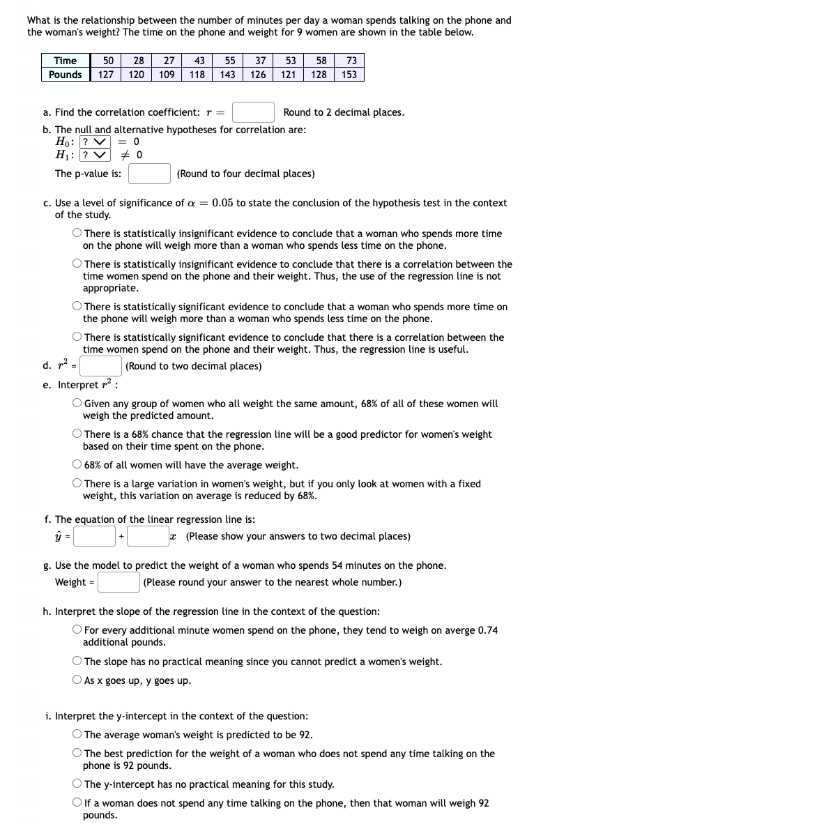

Transcribed Image Text:What is the relationship between the number of minutes per day a woman spends talking on the phone and
the woman's weight? The time on the phone and weight for 9 women are shown in the table below.
Time
50
28
27
43
55
37
53
58 73
Pounds 127 120 109 118 143 126 121
128 153
a. Find the correlation coefficient: r =
Round to 2 decimal places.
b. The null and alternative hypotheses for correlation are:
Ho: ? V = 0
H1: ? V + 0
The p-value is:
(Round to four decimal places)
c. Use a level of significance of a = 0.05 to state the conclusion of the hypothesis test in the context
of the study.
O There is statistically insignificant evidence to conclude that a woman who spends more time
on the phone will weigh more than a woman who spends less time on the phone.
O There is statistically insignificant evidence to conclude that there is a correlation between the
time women spend on the phone and their weight. Thus, the use of the regression line is not
appropriate.
O There is statistically significant evidence to conclude that a woman who spends more time on
the phone will weigh more than a woman who spends less time on the phone.
O There is statistically significant evidence to conclude that there is a correlation between the
time women spend on the phone and their weight. Thus, the regression line is useful.
d. r? =
(Round to two decimal places)
e. Interpret r2 :
O Given any group of women who all weight the same amount, 68% of all of these women will
weigh the predicted amount.
There is a 68% chance that the regression line will be a good predictor for women's weight
based on their time spent on the phone.
O 68% of all women will have the average weight.
O There is a large variation in women's weight, but if you only look at women with a fixed
weight, this variation on average is reduced by 68%.
f. The equation of the linear regression line is:
ŷ =
* (Please show your answers to two decimal places)
g. Use the model to predict the weight of a woman who spends 54 minutes on the phone.
Weight =
(Please round your answer to the nearest whole number.)
h. Interpret the slope of the regression line in the context of the question:
O For every additional minute women spend on the phone, they tend to weigh on averge 0.74
additional pounds.
O The slope has no practical meaning since you cannot predict a women's weight.
O As x goes up, y goes up.
i. Interpret the y-intercept in the context of the question:
O The average woman's weight is predicted to be 92.
O The best prediction for the weight of a woman who does not spend any time talking on the
phone is 92 pounds.
O The y-intercept has no practical meaning for this study.
O If a woman does not spend any time talking on the phone, then that woman will weigh 92
pounds.
Expert Solution
This question has been solved!
Explore an expertly crafted, step-by-step solution for a thorough understanding of key concepts.

Step by stepSolved in 5 steps with 4 images

Knowledge Booster

Similar questions
- You wish to determine if there is a linear correlation between the two variables at a significance level of α=0.01. You have the following bivariate data set. x y 39.3 36.4 52.7 73 50.3 79.8 51.3 71 42 50.8 44.7 74.9 59.2 39.5 54.1 31.6 43.5 90.5 What is the critival value for this hypothesis test?rc.v. = What is the correlation coefficient for this data set?r = Your final conclusion is that... There is insufficient sample evidence to support the claim the there is a correlation between the two variables. There is sufficient sample evidence to support the claim that there is a statistically significant correlation between the two variables. Note: Round to three decimal places when necessary.arrow_forwardA professor at the University of New Hampshire was interested in evaluating the effect of the unemployment rate on the incarceration rate. Using data from 50 states and the District of Columbia (n = 51), the researcher computed the Pearson’s correlation coefficient between the two variables. The results are presented below. Correlations Incarceration Unemployment Incarceration Pearson Correlation 1 .209 Sig. (2-tailed) .142 N 51 51 Unemployment Pearson Correlation .209 1 Sig. (2-tailed) .142 N 51 51 Question What is the sample? What is the dependent variable? What is the independent variable?arrow_forwardYou wish to determine if there is a linear correlation between the two variables at a significance level of α=0.01α=0.01. You have the following bivariate data set. Round to three decimal places. x y 42.5 71 73.7 96 38.5 52.8 42.5 73 40 79.9 62.3 128.8 39.4 106.1 What is the critival value for this hypothesis test?rc.v. = ±± What is the correlation coefficient for this data set?arrow_forward
- 2021arrow_forwardyou are given the following information about x and y. xi independebt varible yi dependent varible 4 12 6 3 2 7 4 6 The sample correlation coefficient equals _____.arrow_forward4 A study was done to look at the relationship between number of lovers college students have had in their lifetimes and their GPAs. The results of the survey are shown below. Lovers 4 8 3 7 0 6 5 6 GPA 2.7 2.3 3.4 2.4 3.5 2.9 2.7 2.8 Find the correlation coefficient: r=r= Round to 2 decimal places. The null and alternative hypotheses for correlation are:H0:H0: ? μ r ρ == 0H1:H1: ? ρ r μ ≠≠ 0 The p-value is: (Round to four decimal places) Use a level of significance of α=0.05α=0.05 to state the conclusion of the hypothesis test in the context of the study. There is statistically insignificant evidence to conclude that there is a correlation between the number of lovers students have had in their lifetimes and their GPA. Thus, the use of the regression line is not appropriate. There is statistically insignificant evidence to conclude that a student who has had more lovers will have a lower GPA than a student who has had fewer lovers. There is statistically…arrow_forward
- ont Paragraph Styles 4. The given table below shows the respective correlation coefficients between two variables with the corresponding p-values. Assume that the target population is composed of all ADZU employees. Required: a) Write the null hypothesis(Ho) and alternative hypothesis (Ha) for each pair of variables as reflected in the table below. b) Decide whether the null hypothesis can be rejected and then discuss the results (at least 15 words) for each pair of variables. Fasting Blood Sugar Level (FBSL) Systolic Blood Pressure (SBP) 0.85 p-value = 0.03 Body Mass Index (BMI) -0.63 p-value=0.005 Focus W Accessibility: Investigate 17 17 43arrow_forwardYou wish to determine if there is a linear correlation between the two variables at a significance level of a = 0.01. You have the following bivariate data set. X y 64.4 45.7 43.9 165.3 63.9 -15.5 65.5 12.6 64 73.9 63 25.9 59.9 34.8 45.1 99.2 What is the critival value for this hypothesis test? rc.v. = What is the correlation coefficient for this data set? r = Your final conclusion is that... O There is insufficient sample evidence to support the claim the there is a correlation between the two variables. There is sufficient sample evidence to support the claim that there is a statistically significant correlation between the two variables.arrow_forwardProvide an interpretation for the following SPSS output: A researcher wanted to test the relationship between number of fries eaten per week and number of vegetables eaten per week by the sample. Number of times Number of times eat fries per eat vegetables week per week Number of times eat fries per Pearson Correlation 1 -.067 week Sig. (2-tailed) .005 N 1750 1750 Number of times eat Pearson Correlation -.067 1 vegetables per week Sig. (2-tailed) N .005 1750 1750 **Correlation is significant at the 0.01 level (2-tailed). Edit View Insert Format Tools Table 12pt v Paragrapharrow_forward
- A professor at the University of New Hampshire was interested in evaluating the effect of the unemployment rate on the incarceration rate. Using data from 50 states and the District of Columbia (n = 51), the researcher computed the Pearson’s correlation coefficient between the two variables. The results are presented below. Correlations Incarceration Unemployment Incarceration Pearson Correlation 1 .209 Sig. (2-tailed) .142 N 51 51 Unemployment Pearson Correlation .209 1 Sig. (2-tailed) .142 N 51 51 Using an alpha level of 0.05 and the four steps of the hypothesis testing process, test the research hypotheses that unemployment increases incarceration. Step 3 Step 4 Based on your decision to step 4 what type of error might you be making?arrow_forwardSubject Extroversion Neuroticism 1 43 49 2 46 53 3 48 67 4 48 57 5 48 56 6 50 48 7 51 60 8 51 41 9 53 51 10 58 47 11 62 41 12 63 51 13 63 30 14 63 28 15 67 55 16 67 47 17 67 39 7. What is the standard error of the correlation coefficient for the association of extroversion and neuroticism in personalities.xls? 8. Carry out a formal t-test for the association between extroversion and neuroticism in personalities.xls. H0: The population correlation coefficient is 0. HA: The population correlation coefficient is not 0. What is the value of the t-statistic corresponding to this test? (Report the absolute value. The t-distribution is symmetric, thus it is easier to compare the absolute value of the t-statistic with the positive values in statistical table C). 9. Carry out a formal t-test for the association between extroversion and neuroticism in personalities.xls. H0: The population correlation coefficient is 0. HA: The population correlation coefficient is not 0. What is the critical…arrow_forward2arrow_forward
arrow_back_ios
SEE MORE QUESTIONS
arrow_forward_ios
Recommended textbooks for you
- MATLAB: An Introduction with ApplicationsStatisticsISBN:9781119256830Author:Amos GilatPublisher:John Wiley & Sons Inc
 Probability and Statistics for Engineering and th...StatisticsISBN:9781305251809Author:Jay L. DevorePublisher:Cengage Learning
 Statistics for The Behavioral Sciences (MindTap C...StatisticsISBN:9781305504912Author:Frederick J Gravetter, Larry B. WallnauPublisher:Cengage Learning
  Elementary Statistics: Picturing the World (7th E...StatisticsISBN:9780134683416Author:Ron Larson, Betsy FarberPublisher:PEARSON
 The Basic Practice of StatisticsStatisticsISBN:9781319042578Author:David S. Moore, William I. Notz, Michael A. FlignerPublisher:W. H. Freeman
 Introduction to the Practice of StatisticsStatisticsISBN:9781319013387Author:David S. Moore, George P. McCabe, Bruce A. CraigPublisher:W. H. Freeman
MATLAB: An Introduction with Applications
Statistics
ISBN:9781119256830
Author:Amos Gilat
Publisher:John Wiley & Sons Inc
Probability and Statistics for Engineering and th...
Statistics
ISBN:9781305251809
Author:Jay L. Devore
Publisher:Cengage Learning
Statistics for The Behavioral Sciences (MindTap C...
Statistics
ISBN:9781305504912
Author:Frederick J Gravetter, Larry B. Wallnau
Publisher:Cengage Learning
Elementary Statistics: Picturing the World (7th E...
Statistics
ISBN:9780134683416
Author:Ron Larson, Betsy Farber
Publisher:PEARSON
The Basic Practice of Statistics
Statistics
ISBN:9781319042578
Author:David S. Moore, William I. Notz, Michael A. Fligner
Publisher:W. H. Freeman
Introduction to the Practice of Statistics
Statistics
ISBN:9781319013387
Author:David S. Moore, George P. McCabe, Bruce A. Craig
Publisher:W. H. Freeman