
ENGR.ECONOMIC ANALYSIS
14th Edition
ISBN: 9780190931919
Author: NEWNAN
Publisher: Oxford University Press
expand_more
expand_more
format_list_bulleted
Question
What does the value for the coefficient mean in the regression analysis of both the company ?
P-Values - how its related to customer satisfaction in the regression analysis of both the company ?
Expert Solution
This question has been solved!
Explore an expertly crafted, step-by-step solution for a thorough understanding of key concepts.
This is a popular solution
Trending nowThis is a popular solution!
Step by stepSolved in 5 steps

Follow-up Questions
Read through expert solutions to related follow-up questions below.
Follow-up Question
Need more explanation by considerinng the data given in snapshots
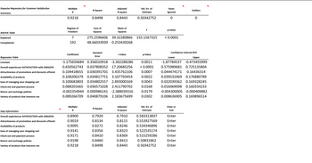
Transcribed Image Text:Stepwise Regression for Customer Satisfaction
Summary
ANOVA Table
Explained
Unexplained
Regression Table
Constant
Overall experiences SATISFACTION with AMAZON
Attractiveness of promotions and discounts offered
Availability of products
Ease of managing your shopping cart
Check-out and payment process
Return and exchange policies
Variety of products that interests me
Step Information
Overall experiences SATISFACTION with AMAZON
Attractiveness of promotions and discounts offered
Availability of products
Ease of managing your shopping cart
Check-out and payment process
Return and exchange policies
Variety of products that interests me
Multiple
R
0.9218
Degrees of
Freedom
7
192
Coefficient
Multiple
R
R-Square
0.8900
0.9019
0.9095
0.9141
0.9171
0.9198
0.9218
0.8498
Sum of
Squares
Standard
Error
Adjusted
R-square
0.8443
R-Square
Mean of
Squares
275.2596606 39.32280866 155.1567325
48.66033939 0.253439268
0.7920
0.8134
0.8272
0.8356
0.8410
0.8460
0.8498
t-Value
-1.175650684 0.356010918 -3.302288286 0.0011
0.650562743 0.037808352 17.20685256 < 0.0001
0.104418655 0.030391701 3.435762106 0.0007
0.108206379 0.034817751 3.107793454 0.0022
0.100683803 0.034802557 2.893000169 0.0043
0.088201665 0.036571028 2.411790702 0.0168
-0.002354944 0.000986141 -2.388039316 0.0179
0.089266709 0.040879106 2.183675699 0.0302
Std. Err. of
Estimate
0.50342752
Adjusted
R-square
F
0.7910
0.8115
0.8246
0.8323
0.8369
0.8413
0.8443
p-Value
Std. Err. of
Estimate
0.583313837
0.553927569
0.534346896
0.522535174
0.515259286
0.50831862
0.50342752
Rows
Ignored
0
p-Value
< 0.0001
Enter or
Exit
Confidence Interval 95%
Lower
Upper
-1.87784537 -0.473455999
0.575989681 0.725135804
0.044474171 0.16436314
0.039531969 0.176880789
0.032039362 0.169328245
0.016069098 0.160334233
-0.004300005 -0.000409882
0.008636905 0.169896514
Enter
Enter
Enter
Outliers
Enter
Enter
Enter
Enter
0
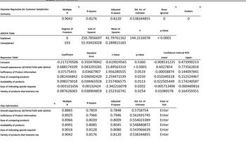
Transcribed Image Text:Stepwise Regression for Customer Satisfaction
Summary
ANOVA Table
Explained
Unexplained
Regression Table
Constant
Overall experiences SATISFACTION with QO010
Sufficiency of Product information
Ease of comparing products
Availability of products
Ease of indicating special requests
Variety of products that interests me
Step Information
Overall experiences SATISFACTION with QO010
Sufficiency of Product information
Ease of comparing products
Availability of products
Ease of indicating special requests
Variety of products that interests me
Multiple
R
0.9042
Degrees of
Freedom
6
193
Coefficient
Multiple
R
R-Square
0.8865
0.8925
0.8966
0.8991
0.9016
0.9042
0.8176
Sum of
Squares
Standard
Error
250.7856697 41.79761162
55.93433028 0.289815183
Adjusted
R-square
0.8120
R-Square
Mean of
Squares
0.7859
0.7966
0.8039
0.8085
0.8128
0.8176
t-Value
-0.217270506 0.350478942 -0.619924565 0.5360
0.688174109 0.043293281 15.89563319 < 0.0001
0.07175455 0.03667907 1.956280555 0.0519
0.081436842 0.036042429 2.259471539 0.0250
0.098373018 0.038465928 2.557406575 0.0113
-0.003101656 0.00132424 -2.342216078 0.0202
0.087626065 0.038904859 2.252316741 0.0254
Adjusted
R-square
Std. Err. of
Estimate
0.7848
0.7946
0.8009
0.8045
0.8080
0.8120
0.538344855
F
144.2216078
p-Value
Std. Err. of
Estimate
0.5758754
0.562691745
0.554023389
0.548880872
0.543966639
0.538344855
Rows
Ignored
0
p-Value
< 0.0001
Outliers
Confidence Interval 95%
Enter or
Exit
0
Lower
Upper
-0.908531225 0.473990213
0.6027854 0.773562818
-0.00058874 0.144097841
0.010349218 0.152524467
0.022505449 0.174240587
-0.005713496 -0.000489816
0.01089278 0.164359351
Enter
Enter
Enter
Enter
Enter
Enter
Solution
by Bartleby Expert
Follow-up Questions
Read through expert solutions to related follow-up questions below.
Follow-up Question
Need more explanation by considerinng the data given in snapshots

Transcribed Image Text:Stepwise Regression for Customer Satisfaction
Summary
ANOVA Table
Explained
Unexplained
Regression Table
Constant
Overall experiences SATISFACTION with AMAZON
Attractiveness of promotions and discounts offered
Availability of products
Ease of managing your shopping cart
Check-out and payment process
Return and exchange policies
Variety of products that interests me
Step Information
Overall experiences SATISFACTION with AMAZON
Attractiveness of promotions and discounts offered
Availability of products
Ease of managing your shopping cart
Check-out and payment process
Return and exchange policies
Variety of products that interests me
Multiple
R
0.9218
Degrees of
Freedom
7
192
Coefficient
Multiple
R
R-Square
0.8900
0.9019
0.9095
0.9141
0.9171
0.9198
0.9218
0.8498
Sum of
Squares
Standard
Error
Adjusted
R-square
0.8443
R-Square
Mean of
Squares
275.2596606 39.32280866 155.1567325
48.66033939 0.253439268
0.7920
0.8134
0.8272
0.8356
0.8410
0.8460
0.8498
t-Value
-1.175650684 0.356010918 -3.302288286 0.0011
0.650562743 0.037808352 17.20685256 < 0.0001
0.104418655 0.030391701 3.435762106 0.0007
0.108206379 0.034817751 3.107793454 0.0022
0.100683803 0.034802557 2.893000169 0.0043
0.088201665 0.036571028 2.411790702 0.0168
-0.002354944 0.000986141 -2.388039316 0.0179
0.089266709 0.040879106 2.183675699 0.0302
Std. Err. of
Estimate
0.50342752
Adjusted
R-square
F
0.7910
0.8115
0.8246
0.8323
0.8369
0.8413
0.8443
p-Value
Std. Err. of
Estimate
0.583313837
0.553927569
0.534346896
0.522535174
0.515259286
0.50831862
0.50342752
Rows
Ignored
0
p-Value
< 0.0001
Enter or
Exit
Confidence Interval 95%
Lower
Upper
-1.87784537 -0.473455999
0.575989681 0.725135804
0.044474171 0.16436314
0.039531969 0.176880789
0.032039362 0.169328245
0.016069098 0.160334233
-0.004300005 -0.000409882
0.008636905 0.169896514
Enter
Enter
Enter
Outliers
Enter
Enter
Enter
Enter
0

Transcribed Image Text:Stepwise Regression for Customer Satisfaction
Summary
ANOVA Table
Explained
Unexplained
Regression Table
Constant
Overall experiences SATISFACTION with QO010
Sufficiency of Product information
Ease of comparing products
Availability of products
Ease of indicating special requests
Variety of products that interests me
Step Information
Overall experiences SATISFACTION with QO010
Sufficiency of Product information
Ease of comparing products
Availability of products
Ease of indicating special requests
Variety of products that interests me
Multiple
R
0.9042
Degrees of
Freedom
6
193
Coefficient
Multiple
R
R-Square
0.8865
0.8925
0.8966
0.8991
0.9016
0.9042
0.8176
Sum of
Squares
Standard
Error
250.7856697 41.79761162
55.93433028 0.289815183
Adjusted
R-square
0.8120
R-Square
Mean of
Squares
0.7859
0.7966
0.8039
0.8085
0.8128
0.8176
t-Value
-0.217270506 0.350478942 -0.619924565 0.5360
0.688174109 0.043293281 15.89563319 < 0.0001
0.07175455 0.03667907 1.956280555 0.0519
0.081436842 0.036042429 2.259471539 0.0250
0.098373018 0.038465928 2.557406575 0.0113
-0.003101656 0.00132424 -2.342216078 0.0202
0.087626065 0.038904859 2.252316741 0.0254
Adjusted
R-square
Std. Err. of
Estimate
0.7848
0.7946
0.8009
0.8045
0.8080
0.8120
0.538344855
F
144.2216078
p-Value
Std. Err. of
Estimate
0.5758754
0.562691745
0.554023389
0.548880872
0.543966639
0.538344855
Rows
Ignored
0
p-Value
< 0.0001
Outliers
Confidence Interval 95%
Enter or
Exit
0
Lower
Upper
-0.908531225 0.473990213
0.6027854 0.773562818
-0.00058874 0.144097841
0.010349218 0.152524467
0.022505449 0.174240587
-0.005713496 -0.000489816
0.01089278 0.164359351
Enter
Enter
Enter
Enter
Enter
Enter
Solution
by Bartleby Expert
Knowledge Booster
Learn more about
Need a deep-dive on the concept behind this application? Look no further. Learn more about this topic, economics and related others by exploring similar questions and additional content below.Similar questions
- I need Explaination based on the answer key answer is D but how. It is econometricsarrow_forwardwages = B1 + B2educ + ßzexper + e where wages denotes hourly wages. We estimate the regression in R and obtain the output ## Coefficients: ## Estimate Std. Error t value Pr(>|t|) ## (Intercept) 2.0 1.0 2 0.0455 * ## educ 0.5 0.5 1 0.3173 ## exper 2.0 0.5 4 6.33e-05 *** ## --- ## Signif. codes: ****' 0. 001 '**' 0.01 **' 0.05 ' 0.1 ' ' 1 Build a 90% confidence interval for B3 using a normal approximation. (Use that if Z ~ N(0, 1) and z1-a satisfies P(Z > z1-a) = a, then zo9 = 1.28, zo95 = 1.64, Z0.975 = 1.96, zo.99 = 2.33, and z0.995 = 2.58). Oa. [2 – 1.64 x (0.5), 2 + 1.64 x (0.5)] O b. [2 – 1.28 × (0.5), 2 + 1.28 x (0.5)] c. [2 – 1.28 x (0.5)², 2 + 1.28 × (0.5)²] O d. [2 – 1.64 × (0.5)², 2 + 1.64 × (0.5)²] O e. [2 – 1.96 × (0.5)², 2 + 1.96 × (0.5)²] O f. [2 – 1.96 × (0.5), 2 + 1.96 × (0.5)]arrow_forwardIn an OLS regression, which value represents the "best" R2 in terms of explained variance in the dependent variable? A. 2.53 B. 16.22 C. .001 D. 0.53arrow_forward
- You estimated a regression with the following output. Source | SS df MS Number of obs = 411 -------------+---------------------------------- F(1, 409) = 4098.54 Model | 22574040.7 1 22574040.7 Prob > F = 0.0000 Residual | 2252702.97 409 5507.83122 R-squared = 0.9093 -------------+---------------------------------- Adj R-squared = 0.9090 Total | 24826743.7 410 60553.0334 Root MSE = 74.215 ------------------------------------------------------------------------------ Y | Coef. Std. Err. t P>|t| [95% Conf. Interval] -------------+---------------------------------------------------------------- X | 6.727341 .1050822 64.02 0.000 6.520772 6.933909 _cons | -.7552724 9.26027 -0.08 0.935 -18.95894 17.44839…arrow_forwardAn analyst working for your firm provided an estimated log-linear demand function based on the natural logarithm of the quantity sold, price, and the average income of consumers. Results are summarized in the following table: SUMMARY OUTPUT Regression Statistics Multiple R R Square Adjusted R Square Standard Error Observations ANOVA Regression Residual Total Intercept LN Price LN Income df 0.968 0.937 0.933 0.003 30 SS MS F 2 0.003637484 0.001818742 202.48598 0.000242516 8.98206E-06 27 29 0.00388 Coefficients Standard Error 0.57 0.00 0.13 0.51 -0.08 0.15 t Stat 0.90 -19.50 1.13 P-value 0.37 0.00 0.27 Significance F 5.55598E-17 Lower 95% -0.65 -0.09 -0.12 How would a 4 percent increase in income impact the demand for your product? Demand would increase by 60 percent. Demand would increase by 0.6 percent. Demand would decrease by 60 percent. Demand would decrease by 0.6 percent. Upper 95% 1.68 -0.07 0.41arrow_forwardQUESTION 10 Answer questions 10 to 16 based on the regression outputs given in Table 1& 2. Table 1 DATA4-1: Data on single family homes in University City community of San Diego, in 1990. price - sale price in thousands of dollars (Range 199. 9 505) sqft - square feet of living area (Range 1065 - 3000) Table 2 Model 1: OLS, using observations 1-14 Dependent variable: price coefficient std. error t-ratio p-value 52. 3509 0.138750 37. 2855 0.0187329 0. 1857 8. 20e-06 *** const sqft 7. 407 Me dependent var Sun squared resid R-squared F(1, 12) Log-likelihood Schwarz criterion 317. 4929 18273. 57 0. 820522 54. 86051 -70. 08421 145. 4465 Hannan-Quinn S.D. dependent var S.E. of regression Adjusted R-squared P-value (F) Akaike criterion 88. 49816 39. 02304 0. 805565 8. 20e-06 144. 1684 144. 0501 There are observations included in this dataset. It is a. data. O 12; cross-sectional 13; time-series data 14; cross-sectional In this regression model, sale price of a single-family house is the. the…arrow_forward
- The dependent variable in the regression in our cost driver analysis is which of the following? Company sales Total overhead cost for the entire period of time Total overhead cost per montharrow_forwardIn the regression equation, what is B0? Group of answer choices the population slope the sample y-intercept the sample slope the population y-interceptarrow_forwardWhen running a ols regression, if my control variables are insignificant via T-test should I keep them in the regression? Are they significant?arrow_forward
arrow_back_ios
SEE MORE QUESTIONS
arrow_forward_ios
Recommended textbooks for you

 Principles of Economics (12th Edition)EconomicsISBN:9780134078779Author:Karl E. Case, Ray C. Fair, Sharon E. OsterPublisher:PEARSON
 Engineering Economy (17th Edition)EconomicsISBN:9780134870069Author:William G. Sullivan, Elin M. Wicks, C. Patrick KoellingPublisher:PEARSON
 Principles of Economics (MindTap Course List)EconomicsISBN:9781305585126Author:N. Gregory MankiwPublisher:Cengage Learning
 Managerial Economics: A Problem Solving ApproachEconomicsISBN:9781337106665Author:Luke M. Froeb, Brian T. McCann, Michael R. Ward, Mike ShorPublisher:Cengage Learning
 Managerial Economics & Business Strategy (Mcgraw-...EconomicsISBN:9781259290619Author:Michael Baye, Jeff PrincePublisher:McGraw-Hill Education


Principles of Economics (12th Edition)
Economics
ISBN:9780134078779
Author:Karl E. Case, Ray C. Fair, Sharon E. Oster
Publisher:PEARSON

Engineering Economy (17th Edition)
Economics
ISBN:9780134870069
Author:William G. Sullivan, Elin M. Wicks, C. Patrick Koelling
Publisher:PEARSON

Principles of Economics (MindTap Course List)
Economics
ISBN:9781305585126
Author:N. Gregory Mankiw
Publisher:Cengage Learning

Managerial Economics: A Problem Solving Approach
Economics
ISBN:9781337106665
Author:Luke M. Froeb, Brian T. McCann, Michael R. Ward, Mike Shor
Publisher:Cengage Learning

Managerial Economics & Business Strategy (Mcgraw-...
Economics
ISBN:9781259290619
Author:Michael Baye, Jeff Prince
Publisher:McGraw-Hill Education